Autoencoders, VAEs, and GANs on digits

In Posts 21 to 24 we built the MNIST pipeline the hard way: convolutional layers, training loops, and a digit classifier that reads a 28 by 28 image and names the class. Every one of those models looked at an image and produced a label. This post turns the arrow around. We ask the network to produce the image itself, and the whole exercise becomes a study in how much of a digit you can throw away and still get it back. The through-line is compression and its cost: every model here squeezes a digit into a small code and then pays a price to reconstruct it, and the size of that price tells us what the model actually learned. Our plain autoencoder lands at a validation mean squared error (MSE, the average squared pixel difference) of 0.06489 per pixel, 3.1 percent better than the mean-image baseline. That small number is the first sign of how hard generation is.

We work on MNIST throughout, the same 70,000 grayscale digits from torchvision, and we keep every model small enough to train on a CPU in seconds. The point is not to win a benchmark. The point is to watch the reconstruction error, the KL term (how far the code distribution sits from a standard normal), and sample diversity move as we change the objective, and to read what each number says about the code the model built.

What the digits look like

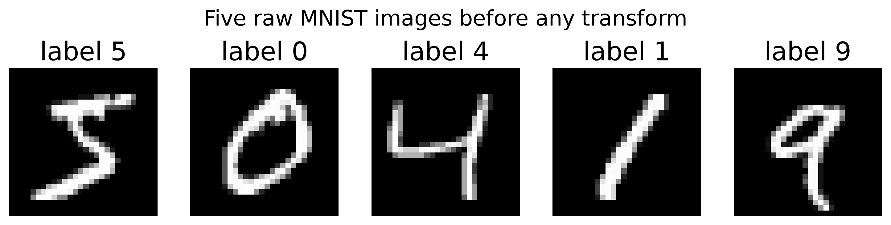
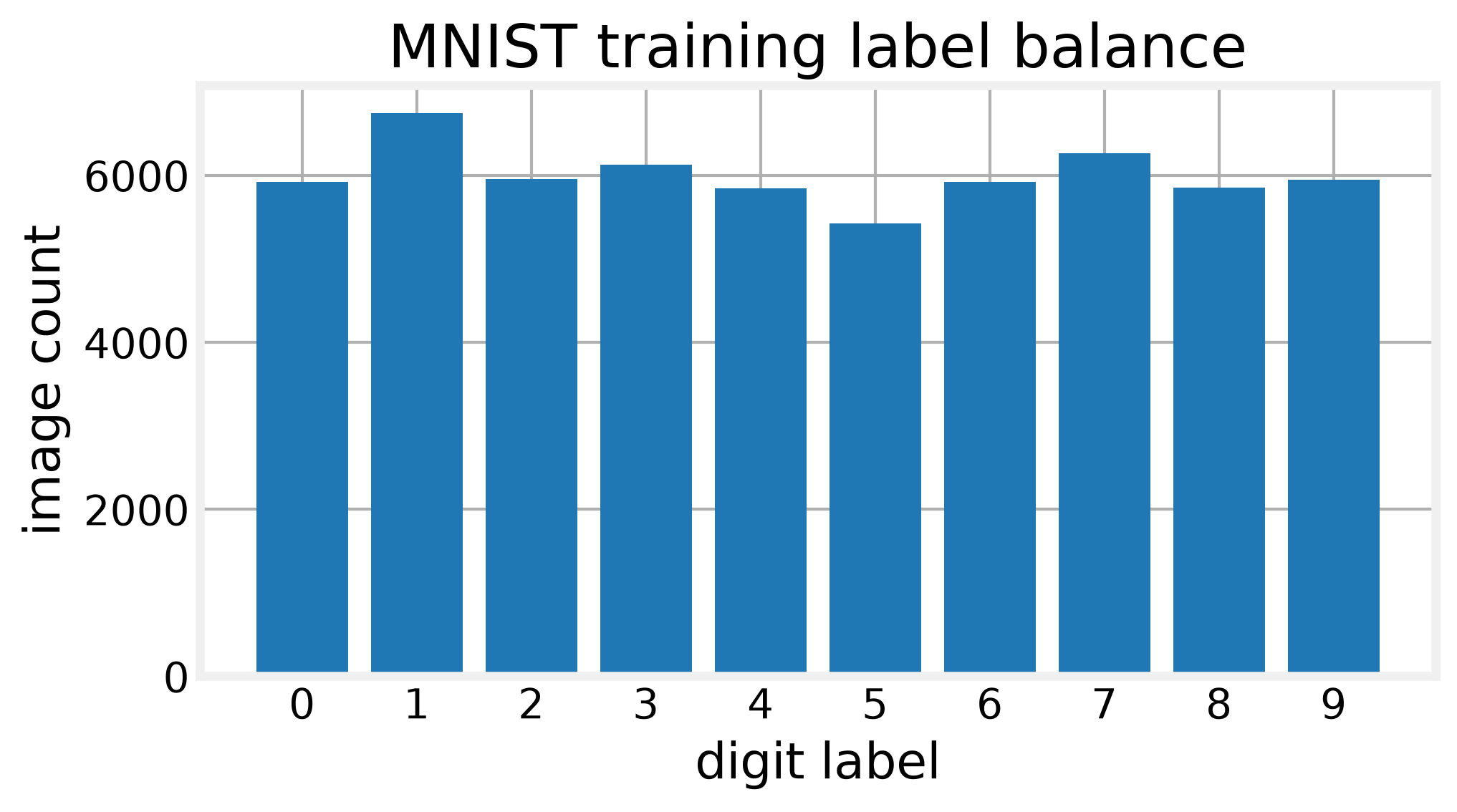
Before any model, we look at the data. The images are 28 by 28 with a single channel, so flattening to 784 values is safe, and the labels run from 0 to 9 with no missing values in either images or labels. The class balance is close to uniform, with digit 1 the most common at 0.112 of the training set and digit 5 the rarest at 0.090, which means label conditioning later will have roughly equal material for every class.

The pixel histogram is the finding that shapes every model choice. About 80.8 percent of pixel values are exactly zero, so the images are mostly empty canvas with a few bright strokes. That sparsity is why we put a sigmoid on every decoder output and score reconstruction with binary cross entropy in the VAE: the target is effectively a soft mask of where ink sits.

We also check for leakage. Hashing every training image finds zero exact duplicates and zero train images that also appear in the test set, so the clean pool stays at all 60,000 images. From that pool we draw a fixed 8,000-image training split and a 2,000-image validation split with seed 42, and every model in the post sees the same split. A mean-image baseline sets the floor: predicting the average digit for every input gives a validation MSE of 0.06696 per pixel, and no autoencoder is allowed to do worse.

A per-class glance shows the shared stroke vocabulary.

Autoencoders

An autoencoder has two functions back to back. The encoder maps a 784-value image to a small latent code, a compressed stand-in for the image, here 32 numbers, and the decoder maps that code back to 784 values. If the reconstruction is good, the code must have kept whatever mattered. We train three variants on the same split: a plain autoencoder, a denoising autoencoder version that sees inputs corrupted with Gaussian noise of sigma 0.35 and must return the clean digit, and a sparse autoencoder version that adds an L1 penalty (a cost on the absolute size of the code values) with weight lambda 0.01.

def add_noise(x, sigma=0.35):
    return torch.clamp(x + sigma * torch.randn_like(x), 0.0, 1.0)

# Denoising: feed the noisy copy, score against the clean target
inp = add_noise(xb) if denoise else xb
out, z = model(inp)
recon = F.mse_loss(out, xb, reduction='mean')
loss = recon + sparse_lambda * z.abs().mean()

All three train in 0.7 seconds total for one epoch each. The plain autoencoder reaches a validation MSE of 0.06489, the sparse version 0.06235, and the denoising version 0.07068 when scored on clean inputs. That last number looks like a loss until we score it the way it was trained: on noisy inputs the plain model gives 0.06591 and the denoising model gives 0.06911, so denoising did not buy us accuracy here, it bought us a different kind of noise tolerance that a single epoch on 8,000 images is too short to show as a clean win. The sparse penalty does exactly what it promises on the code itself, dropping the mean absolute latent value from 4.589 to 0.641.