Learning representations without labels

In the last three posts we built classifiers the ordinary way: labeled images in, cross-entropy out, accuracy on the test set. That recipe assumes every image arrives with a tag, and in the real world most images do not. This post builds a model that learns from unlabeled pictures instead, then checks what it learned by freezing the network and training a tiny classifier on top. The through-line is a simple one: a good representation is a map where things that belong together land close together, and we can draw that map without ever seeing a label. Our SimCLR run on 6,000 unlabeled CIFAR-10 images drives its loss from 4.671 on the first batch down to a mean of 3.859 over the last ten steps.

We work with CIFAR-10, the same 60,000 color images we have used throughout the series, each 32 by 32 pixels. The labels exist, but we hide them during pretraining and only bring them back to score the frozen features. The notebook runs on a laptop budget: 6,000 unlabeled images for pretraining, 3,000 disjoint labeled images to fit a probe, and 1,000 test images to score it. Everything below reproduces on a single GPU in seconds, not hours.

What the data tells us

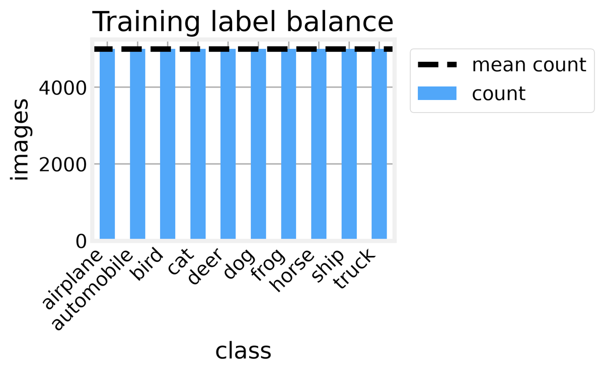
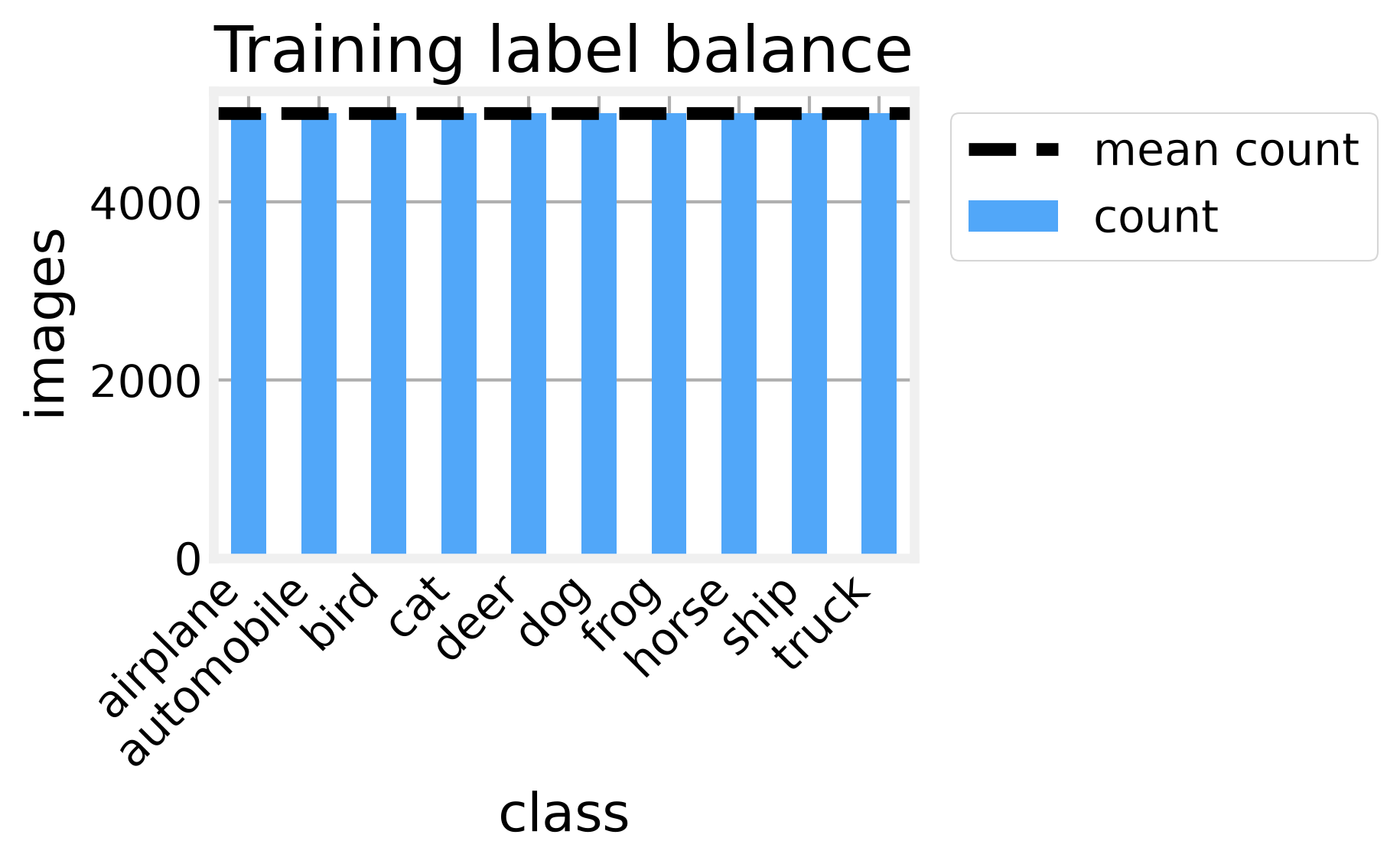
Before any transform we look at the raw pixels, because the augmentation strength and the split policy both depend on what we see. The 50,000-image training split is balanced at 5,000 per class, with 10,000 test images held out, so the base rate for the later linear probe, meaning the score from always guessing one class, is 0.10. That is the floor every number below has to beat.

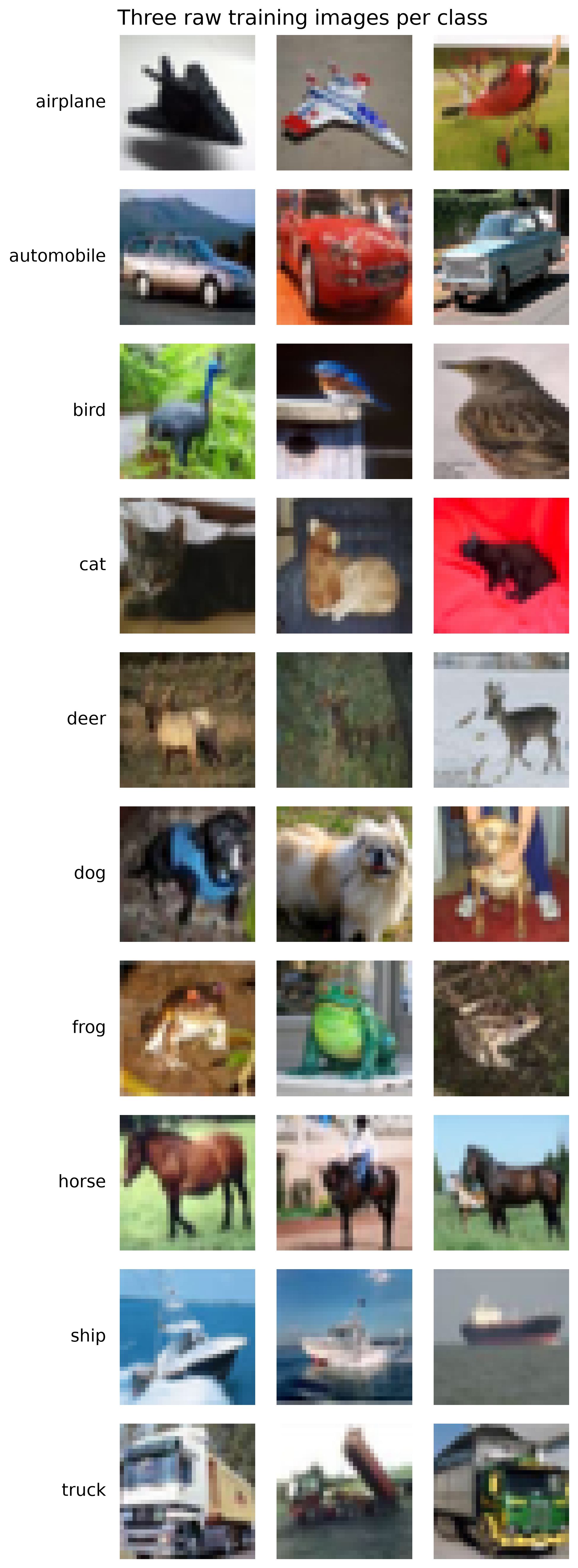
The images are small and noisy, and the per-class rows show how much shape and color vary within a single label. A dog can be dark or bright, centered or off to the side. That variability is exactly what we want the representation to ignore.

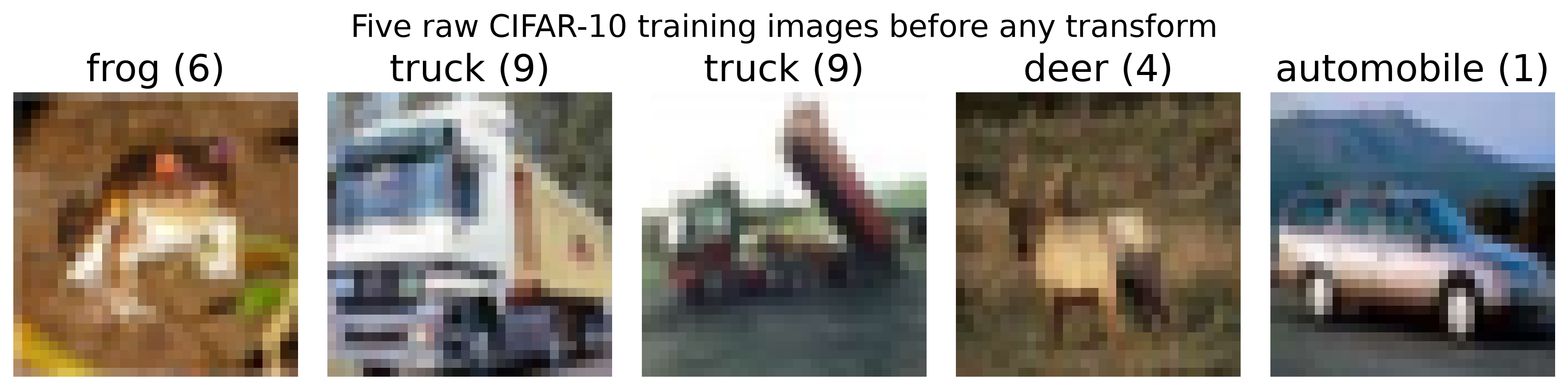
We also check for duplicates and leakage. Hashing a 10,000-image sample of the training set finds zero exact duplicates, and hashing a 2,000-image sample of the test set finds zero overlaps with the training hashes. So we keep the images as they are and guard against leakage by splitting on disjoint indices rather than by deduplication.

The pixel values cover the full 0 to 255 range with a mean of 122.46 and a standard deviation of 63.92, and the per-image means run from 39.34 to 230.39. Some images are very dark, some very bright. That spread is why we normalize with the CIFAR-10 statistics and why we lean on strong crop and color augmentations: the model should see the same object under wildly different lighting and still place it in the same spot.

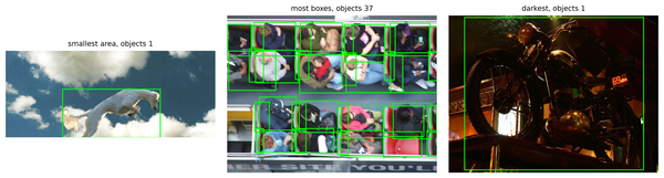
The three odd samples below are the hard cases. Strong color and contrast shifts can hide the shape cues that separate a cat from a dog, so a representation that survives these is one worth keeping. With the data understood, we turn to the first way of drawing the map.

Pulling views together

Contrastive learning takes one image, makes two augmented views of it, and trains the network so those two views land close in representation space while views of other images land far away. The loss that does this is InfoNCE, a softmax over similarity scores where the positive pair is the correct class and every other image in the batch is a negative. SimCLR is the canonical version of this idea: two views, a large batch, and a projection head on top of the encoder, where the projection head is a small feed-forward block that maps encoder features into the contrastive space.

The upgrade over a plain classifier is to declare the two-view dataset and the loss as their own pieces, so one definition drives the whole loop. Here is the loss:

def info_nce_loss(z1, z2, temperature=0.5):
    z1 = F.normalize(z1, dim=1)
    z2 = F.normalize(z2, dim=1)
    logits = torch.cat([z1 @ z2.T, z2 @ z1.T], dim=0) / temperature
    labels = torch.arange(z1.size(0), device=z1.device)
    labels = torch.cat([labels, labels], dim=0)
    return F.cross_entropy(logits, labels)  # positive pair is the diagonal

The two normalized view matrices are multiplied to give a batch-by-batch similarity matrix, scaled by a temperature of 0.5, and the cross-entropy target is the diagonal: each view should match its partner and nothing else. The temperature controls how sharply the softmax punishes near-misses, and 0.5 is a reasonable default for small images.