Kernels, margins, and ensembles

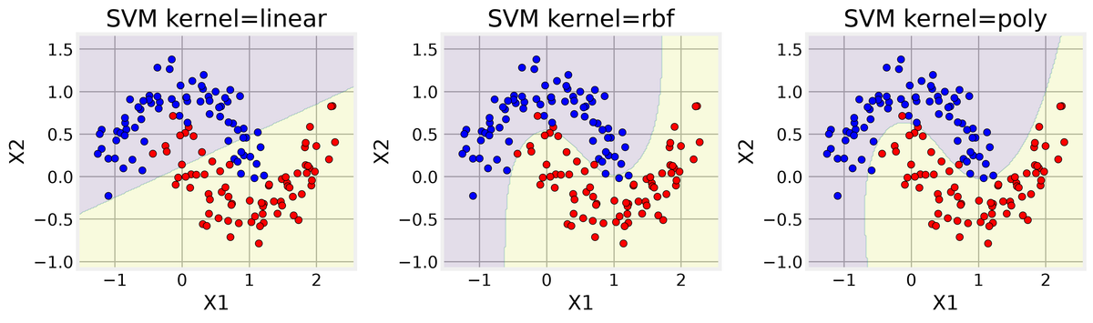
In Posts 11 through 13 we built classifiers that draw boundaries directly, fitting logistic curves and trees to the Adult Census Income data. This post takes the opposite route and then the long way around: we start with generative classifiers that model how each income class produces its features, pivot to Support Vector Machines that hunt for the widest possible margin between classes, and finish by asking whether combining many weak models can beat any single strong one. The through-line is a simple question we keep asking at every step: what does this model actually see when it looks at a row of census data? By the end we have an answer measured by AUC, the area under the receiver operating characteristic curve, which tells how often the model ranks a random above-50K row above a random at-or-below-50K row. 0.5 is chance, 1.0 is perfect. The best single number lands at 0.907.
The dataset is the UCI Adult Census Income table, 32,561 rows after download, each describing a person's age, education, occupation, and weekly hours against a binary label of whether they earn over 50K. After dropping the 24 duplicate rows, the cleaned frame has 32,537 rows. From that cleaned frame we take a stratified 25 percent sample of 8,134 rows, meaning the sample preserves the same 75.9/24.1 class split as the full data, and we hold out 1,627 rows for every evaluation that follows.
What the data says first
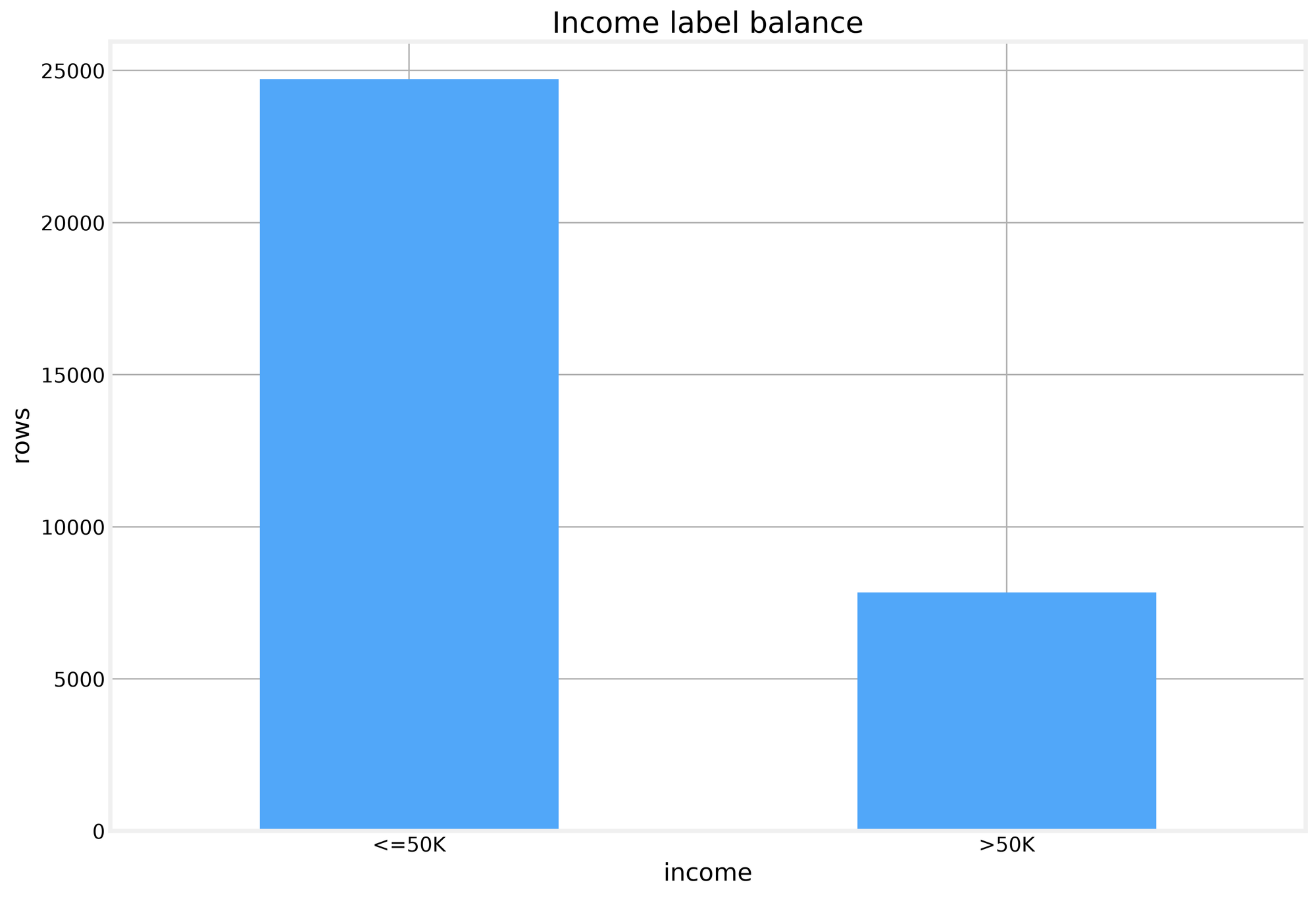
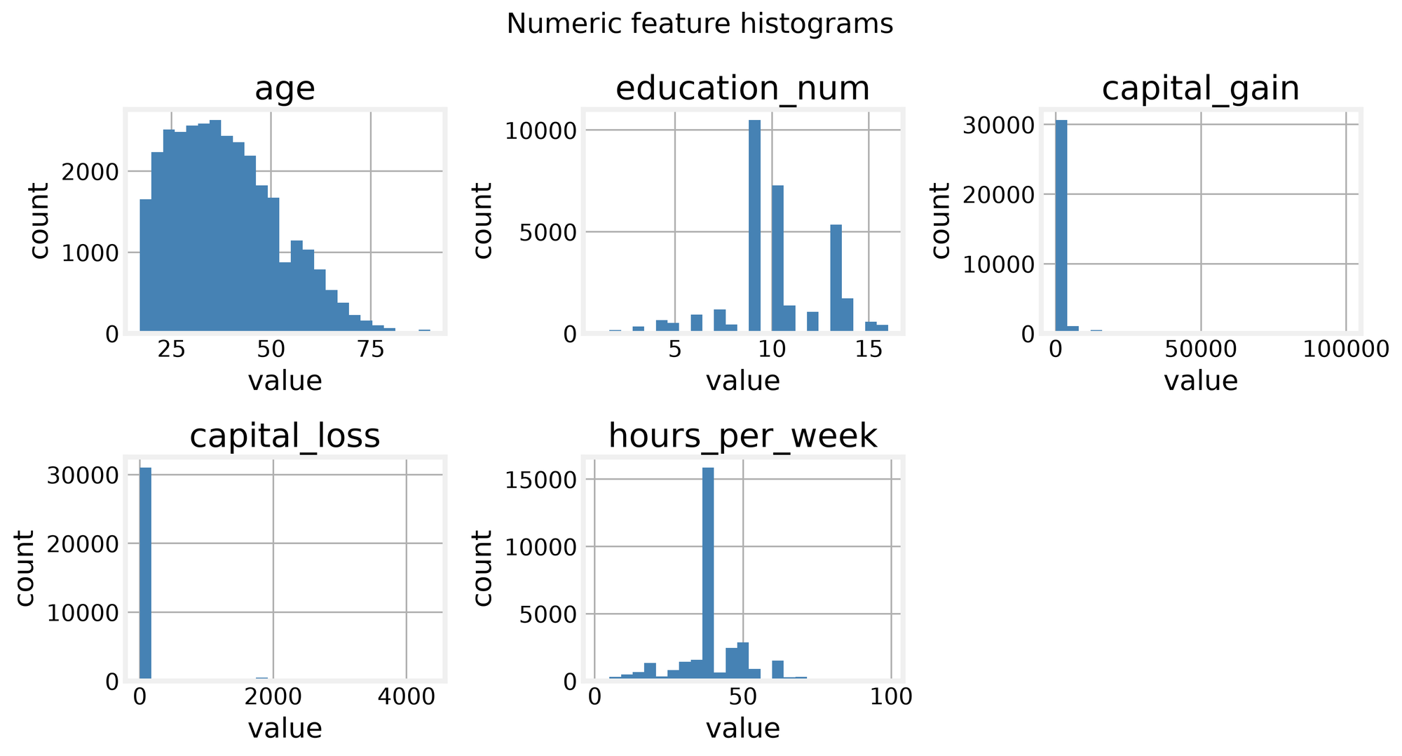
Before any model sees a row, we need an honest picture of what we are predicting. The label balance is the first finding that shapes everything: 75.9 percent of rows earn at most 50K, so a model that predicts the majority class for every row scores 0.759 accuracy. Any classifier worth reporting has to clear that floor. The second finding is where the missing values live. Only three categorical fields, workclass, occupation, and native_country, contain gaps, and we fill them with an explicit Unknown category rather than dropping rows. The third finding is quieter but matters for the ensembles later: capital_gain and capital_loss are heavily right skewed with most values at zero, while hours_per_week clusters near 40 with a long tail of longer weeks.
The histograms show the skew we expected, but the correlation matrix tells a cleaner story. The numeric features barely correlate with each other, which means the signal for high income has to come from combinations of features rather than any single one. That observation will return when we reach the kernel methods.
We also note that education_num is an ordinal coding of education, so we model with it alone and leave the redundant education string out.
Generative classifiers
Generative classifiers take a different stance from the discriminative models we built before. Instead of drawing a boundary directly, they model the probability of the features given each class, then invert with Bayes rule to get the class probability. We test five of them: Gaussian Naive Bayes, Multinomial Naive Bayes, Bernoulli Naive Bayes, Linear Discriminant Analysis, and Quadratic Discriminant Analysis. The contrast between discriminative and generative approaches is the real lesson: discriminative models ask where the boundary lies, generative models ask how each class produces its data.
The implementation is a single evaluation loop that fits each model and records accuracy, AUC, and fit time. The preprocessing pipeline scales the five numeric features to [0, 1] and one-hot encodes the seven categorical fields, turning each category into its own 0/1 column, producing 90 features total. We define the five model instances that the loop will compare as follows.
generative_models = [
    ('gaussian_naive_bayes', GaussianNB()),
    ('multinomial_naive_bayes', MultinomialNB()),
    ('bernoulli_naive_bayes', BernoulliNB(binarize=0.5)),
    ('linear_discriminant_analysis', LinearDiscriminantAnalysis()),
    ('quadratic_discriminant_analysis', QuadraticDiscriminantAnalysis(reg_param=0.01))
]
The results split cleanly. Gaussian Naive Bayes collapses to 0.316 accuracy with an AUC of 0.620, because its Gaussian assumption on the skewed capital fields is badly wrong. Multinomial Naive Bayes recovers to 0.763 accuracy and 0.854 AUC, and Bernoulli Naive Bayes lands at 0.738 accuracy and 0.840 AUC. Linear Discriminant Analysis is the strongest generative model at 0.822 accuracy and 0.878 AUC, while Quadratic Discriminant Analysis trails at 0.735 accuracy and 0.854 AUC. The pattern is clear: the naive Bayes models pay for conditional independence, LDA's pooled covariance makes it the strongest generative model, and QDA's per-class covariance overtunes and trails.