Deep reinforcement learning for control

In Post 35 we solved small control problems with a table. Every state got its own row, every action its own column, and value iteration filled the cells until the numbers stopped moving. That worked while the table fit in memory, but once a state is a vector of four floats or a continuous angle, the table stops existing, so this post builds the machinery that replaces it: neural networks that stand in for the table, policies that are optimized directly, and the trust-region and continuous-control methods that make those policies trainable. The concrete result we reach is a Deep Q-Network (DQN) on CartPole that scores 45.80 against a random baseline of 25.22, and a REINFORCE agent with a baseline that reaches 40.70 on the same environment.
The through-line for the whole post is the gap between random and learned. Every environment gives us a floor for free, the return a coin-flipping policy collects, and every method we build has to clear that floor by a margin we can measure. When a method fails to clear it, the gap tells us exactly how much the method still has to learn.
We work with three Gymnasium classic control environments. CartPole-v1 has a 4-dimensional observation and 2 discrete actions. LunarLander-v2 has an 8-dimensional observation and 4 discrete actions. Pendulum-v1 has a 3-dimensional observation and a single continuous action. All three generate episodes on demand, so there is no dataset to download and every rollout is cheap enough to run on a laptop CPU.
The floor we have to beat
Before training anything, we need to know what random looks like. We ran 100 episodes per environment with a uniformly random policy and recorded the returns. CartPole returns ranged from 9.0 to 87.0 with a mean of 25.22, and the episode length matched the return exactly because every step pays a reward of 1.0. Pendulum returned between -1855.31 and -743.84 with a mean of -1221.86, and every episode ran the full 200 steps because the environment never terminates early. The two scales are not comparable, which is why we normalize advantages before any policy update.
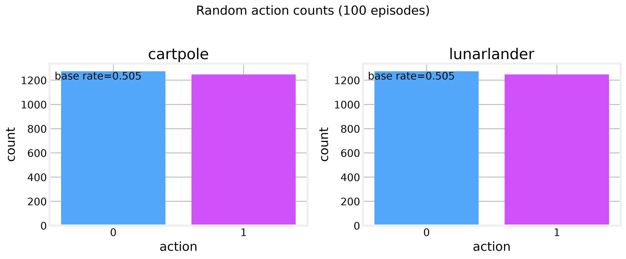
The histogram makes the CartPole floor concrete. Random play clusters near 22 steps with a long right tail, so a learned policy that averages 45 is doing real work. The Pendulum distribution is a wide band of large negative numbers, spanning the full -1855.31 to -743.84 range, which tells us the reward scale is punishing and the policy has to learn to hold the pendulum upright rather than just survive.
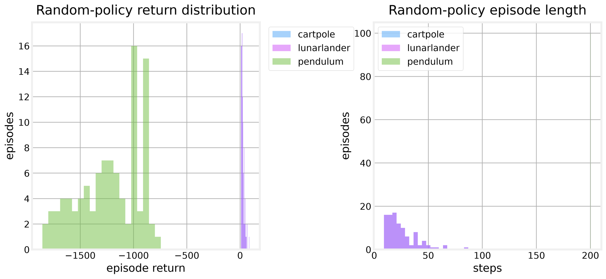
The action counts confirm that random play is close to uniform. CartPole splits near 50/50 and LunarLander spreads across its four actions, so no action-prior correction is needed and no class weighting is needed. We hold out evaluation seeds so random-policy measurements never overlap with training seeds.
Deep value learning
The first idea is to keep Q-learning but replace the table with a network. Function approximation in RL lets us handle continuous states, but it can trigger The deadly triad: function approximation, bootstrapping (updating toward the network's own estimate), and off-policy data (transitions from older policies) can combine to make the value estimates diverge. DQN stabilizes the triad with two tricks. A Replay buffer breaks the correlation between consecutive transitions by sampling random minibatches, and a Target network gives the bootstrap target a slowly moving anchor instead of a value that chases itself.
Double DQN fixes a subtler problem. The max over next-state values in vanilla DQN is biased upward because the same network both selects and evaluates the best action. Double DQN selects the next action with the online network and evaluates it with the target network, which removes most of that bias. Dueling networks split the output into a state value and a per-action advantage, so the network can learn that some states are good regardless of which action we take. Prioritized experience replay samples transitions with large errors more often, which focuses learning where it is most wrong.
The core of the update is the target calculation and the loss. We compute the current Q-value, pick the next action with the online net, evaluate it with the target net, and regress toward the bootstrapped target.
q = self.online(states).gather(1, actions)
with torch.no_grad():
    next_actions = self.online(next_states).argmax(dim=1, keepdim=True)  # Double DQN selection
    next_q = self.target(next_states).gather(1, next_actions)             # target net evaluation
    target = rewards + self.gamma * (1.0 - dones) * next_q
loss = self.loss_fn(q, target)
We trained a dueling double DQN on CartPole for 200 episodes with a replay buffer of 10,000 transitions, a batch size of 64, and a target sync every 200 steps. The last-20 training return averaged 26.15 and the mean Huber loss was 0.3094. That training figure sits near the random floor because training returns include epsilon-greedy exploration, while the held-out evaluation runs the greedy policy. On that held-out evaluation with 10 episodes the greedy agent scored 45.80 against the random baseline of 25.22. That gap is the whole lesson for value learning: the network learned a policy that survives roughly twice as long as random play, and the loss curve stayed flat enough that the target network and replay buffer did their job.