Sequence-to-sequence models with attention

In Posts 25 and 26 we built up the machinery of sequence models, one token at a time, and watched a recurrent network carry a hidden state forward through a sentence. That works fine when the input and the output are the same length. Translation is not so polite. A German sentence can be shorter or longer than its English source, and the words do not line up one to one. This post builds the model that handles that mismatch: a GRU encoder-decoder with Bahdanau attention, trained on 4,000 English-German pairs, reaching a free-running (feeding the model its own predictions instead of gold tokens) test token accuracy of 0.315. The through-line we will follow is alignment, the quiet question of which source words a decoder should be looking at when it writes each target word. Attention is the answer, and the whole post is about learning to see it.

We work with Multi30k, a small parallel corpus (the same captions in English and German) of about 30,000 short image captions. Short sentences keep the demo honest: a single small GPU can train it in a few seconds per epoch, and the attention weights are small enough to read. We subsample to 4,000 training pairs, 500 validation, and 500 test, with a fixed seed so the splits are disjoint.

Reading the corpus first

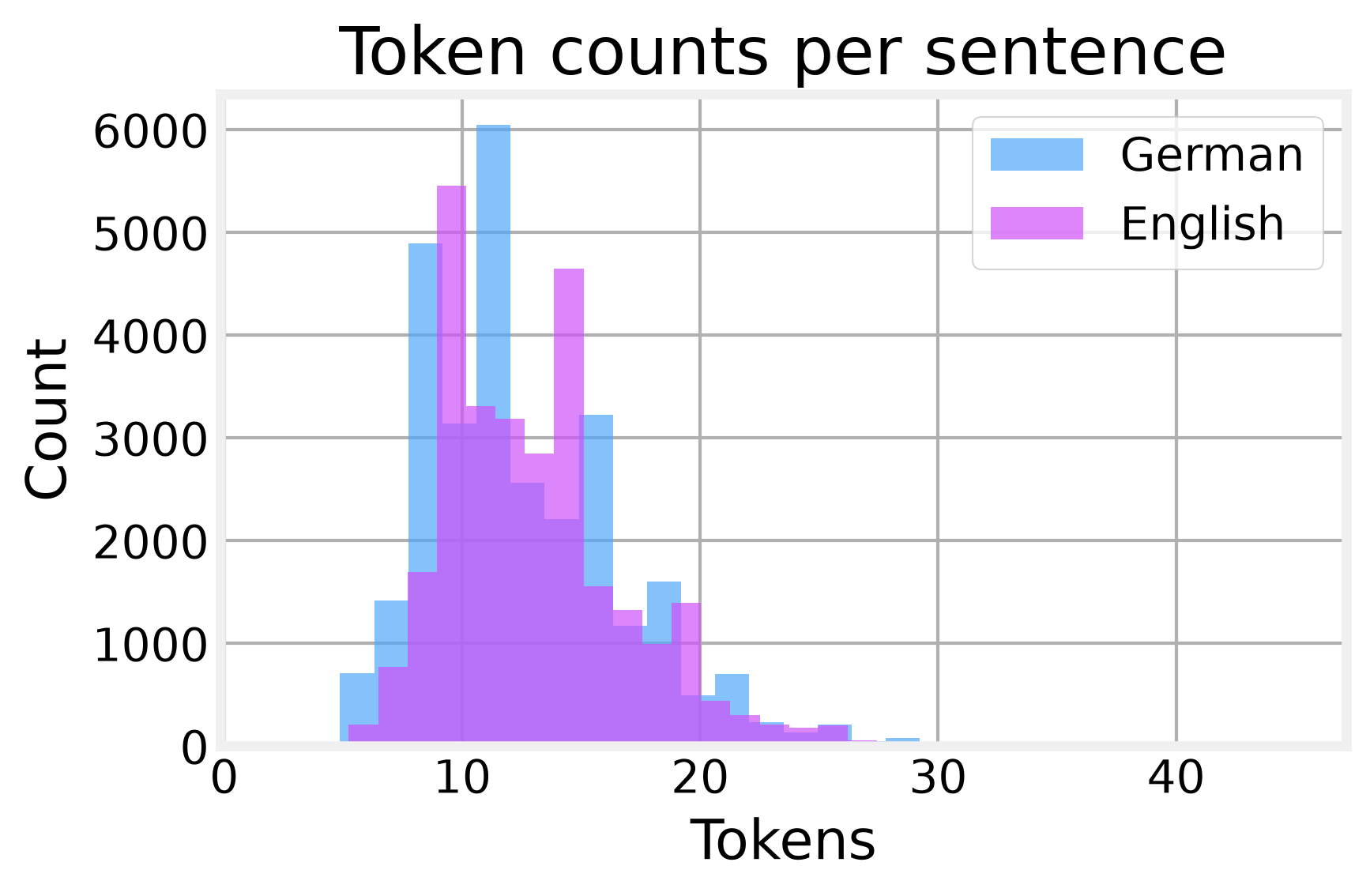
Before building anything, we look at what we are translating. We tokenize with a simple regex that splits words and punctuation, then count. English sentences run a mean of 13.1 tokens with a median of 12 and a max of 41. German is close behind at 12.6 mean, 12 median, 45 max. A max length of 50 covers essentially everything, so that is our cap.

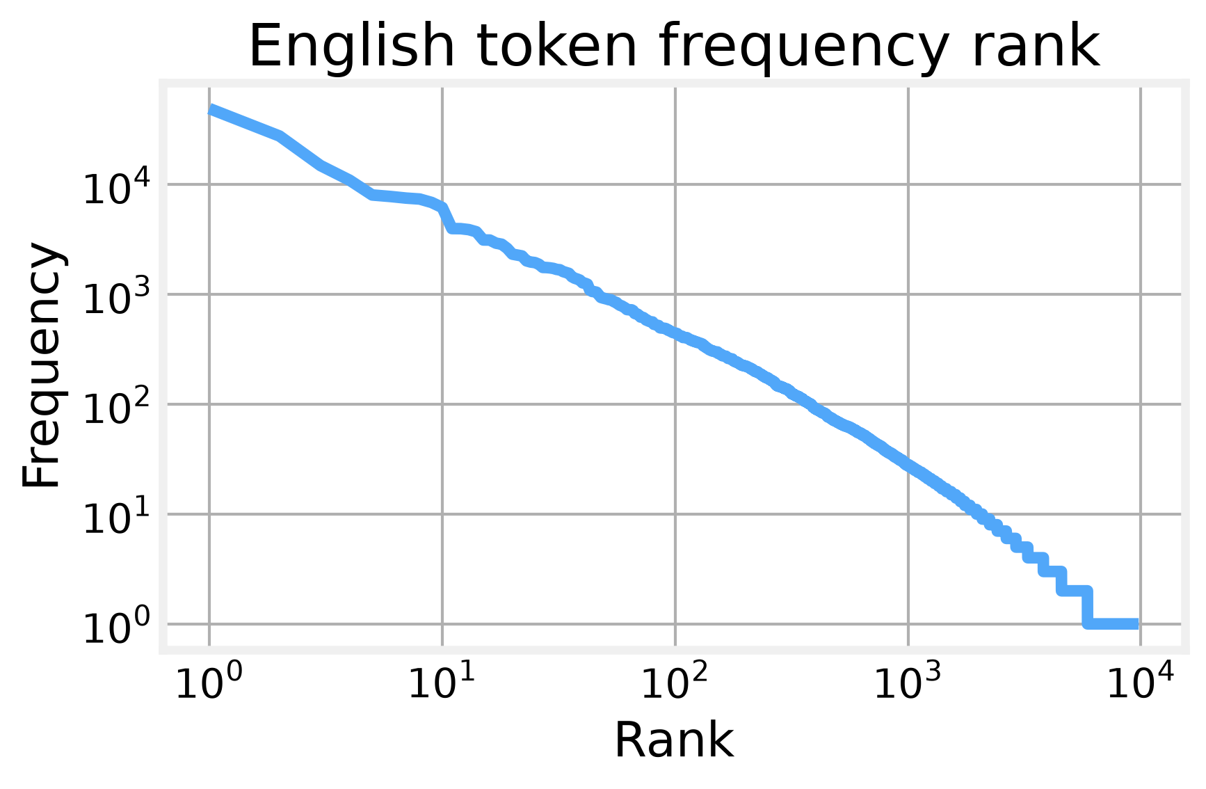
The vocabularies tell us how much of the language we can afford to keep. On the 4,000-pair training split, before the frequency cutoff, we count 9,779 unique English word forms (types) and 17,911 German types, and the frequencies follow a power law, which is the familiar long tail of rare words. Figure 1 plots frequency by rank on log-log axes.

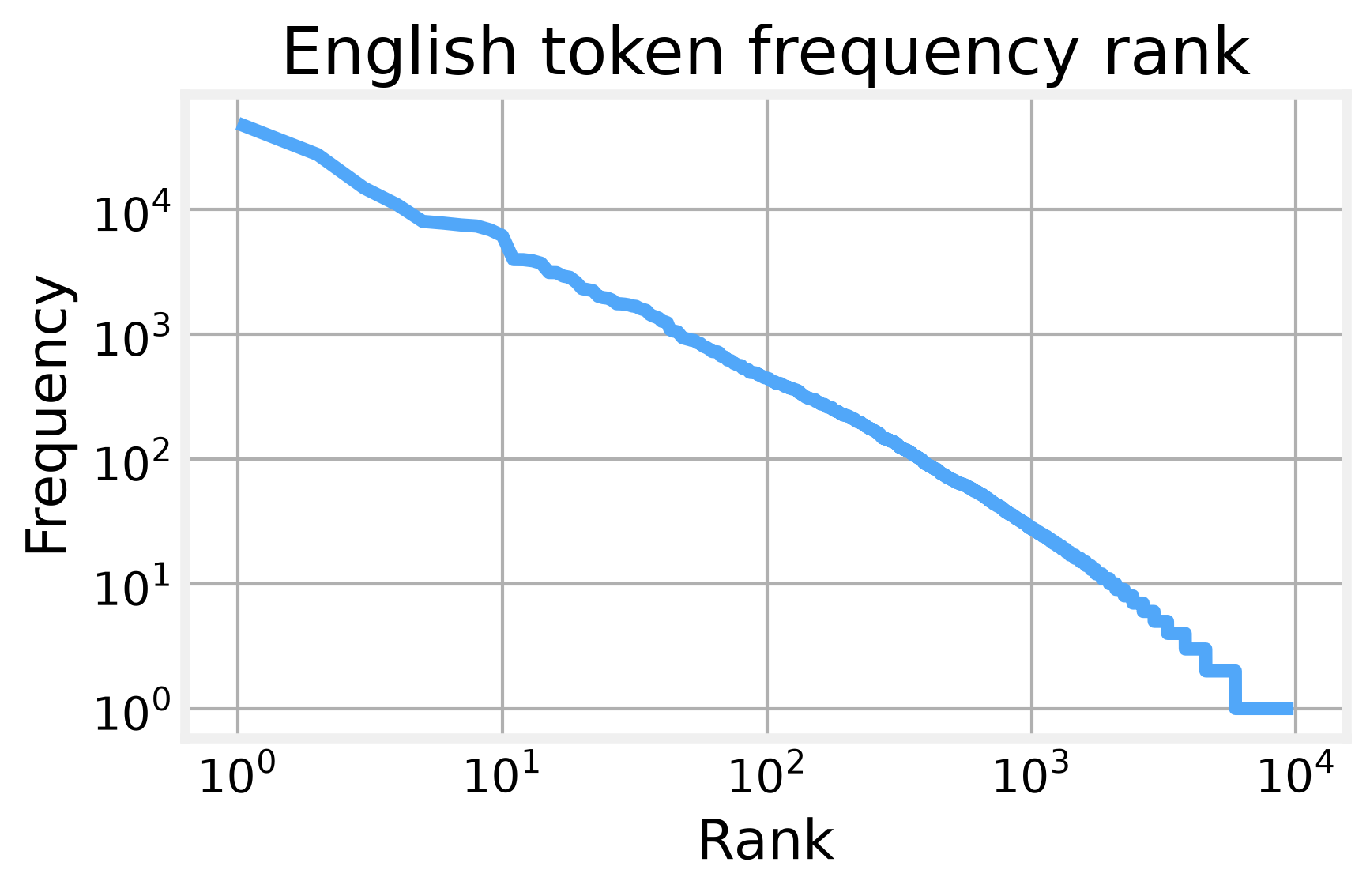
That tail is why we set a minimum frequency of 2 and accept that rare words collapse into <unk>. On the validation split the out-of-vocabulary rate lands near about 5 percent for English and 6 percent for German, so the cutoff costs us little. We also check for leakage: only 3 duplicate pairs in training, and just 1 English sentence shared between train and validation. We drop the duplicates and move on. The length distribution is broad and unimodal, and the most common German length is 11 tokens, covering 10.9 percent of examples. That concentration is too low for length alone to predict much. Figure 2 plots the English and German length histograms.

Those findings set the hyperparameters we carry forward: max length 50, embedding size 128, minimum frequency 2. With the data understood, we can build the recurrent core.

Recurrent models

The recurrent neural network (RNN) reads a sequence one step at a time and folds each token into a hidden state. Backpropagation through time (BPTT) is how it learns: unroll the recurrence and apply the chain rule across every step. The trouble is that gradients multiply through those steps, so long sequences either explode or vanish. GRU networks tame this with an update gate and a reset gate, and they get most of the benefit of the more elaborate LSTM gates while keeping fewer knobs; bidirectional RNNs run two recurrences in opposite directions and concatenate the results, so each position sees both its past and its future.

We can confirm the shapes and the gradient behavior in a few lines. A forward GRU over a batch of 3 sequences of length 7 with hidden size 16 returns outputs of shape (7, 3, 16) and a hidden state of (1, 3, 16). Make it bidirectional and the hidden size doubles to 32, because two directions are stacked. The gradient check is the more instructive one:

w = torch.tensor(1.0, requires_grad=True)
h0 = w * torch.tensor(2.0)
h1 = w * h0 + torch.tensor(3.0)   # two time steps chained through w
h1.sum().backward()
print(w.grad.item())              # 4.0, the sum of both paths

The gradient is 4.0: h1 expands to 2w² + 3, so the derivative is 4w, which is 4 at w=1. The added 3 contributes no gradient. That sum over time steps is the whole story of why long sequences misbehave: each step contributes another factor, and the product either shrinks to nothing or blows up. Gradient clipping at 1.0 in the training loop is our seatbelt against the blow-up. With the recurrent core in hand, we can wire an encoder to a decoder.