Probability and estimation on census data

In the last post we wrangled the Adult Census Income dataset into a clean, analysis-ready form. Now we turn that clean data into a laboratory for the core ideas of probability and estimation: Bayes' theorem, the distributions that describe real populations, the limit theorems that justify our confidence, and the estimators that turn data into decisions. By the end, we will have estimated the probability that a person earns more than $50,000 per year, measured how precise that estimate is, and confirmed that our estimator is as good as theory says it can be. The through-line is a single question: how well can we know the income rate from a sample, and how do we prove we know it?
The dataset as our probability lab
The Adult Census Income dataset holds 32,561 records after dropping the few rows with missing values. Each row is a person, and the target is a binary variable: income above or below $50,000. That binary outcome makes the dataset a natural home for Bernoulli trials, and the large sample size lets us watch the Law of Large Numbers and the Central Limit Theorem unfold in real data.
Our first look at the data told us the baseline. About 24.9 percent of the sample earns more than $50,000. Age follows a roughly Gaussian distribution with mean 38.4 years and standard deviation 13.1. The correlation between numeric features is weak—the largest absolute value is around 0.1. These findings set expectations: the income rate is the single number we will estimate, and the near-normality of age will let us demonstrate the CLT cleanly.
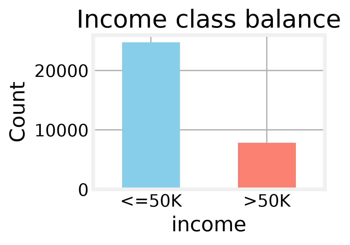
The bar chart shows the imbalance: 75.1% earn $50,000 or less; 24.9% earn more. That 24.9 percent is our base rate, and it will serve as the population parameter throughout the post.
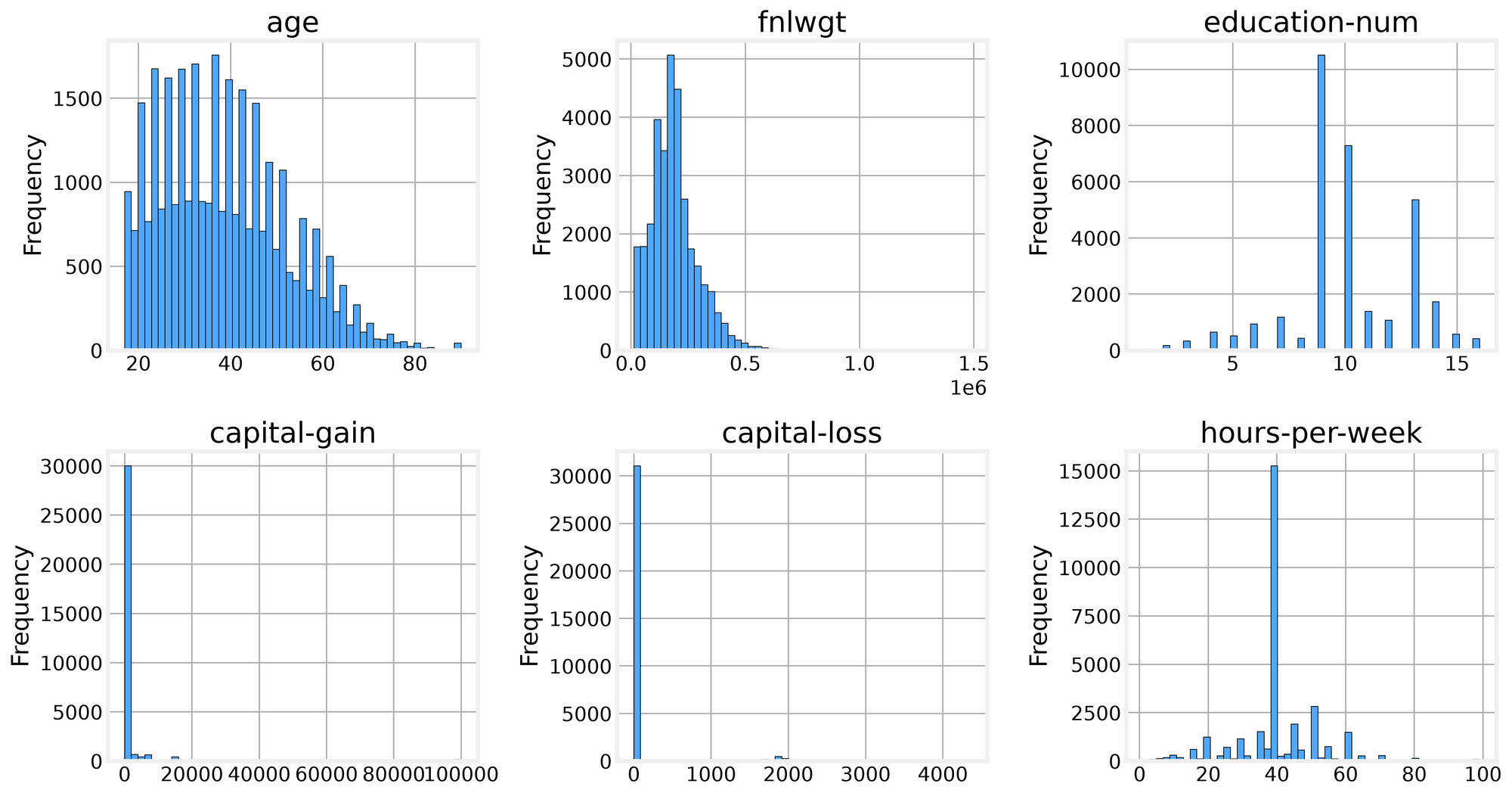
Age and hours-per-week look roughly symmetric. Capital-gain and capital-loss are spike-and-zero distributions, which we will not model here but note as a reminder that real data rarely matches textbook examples.
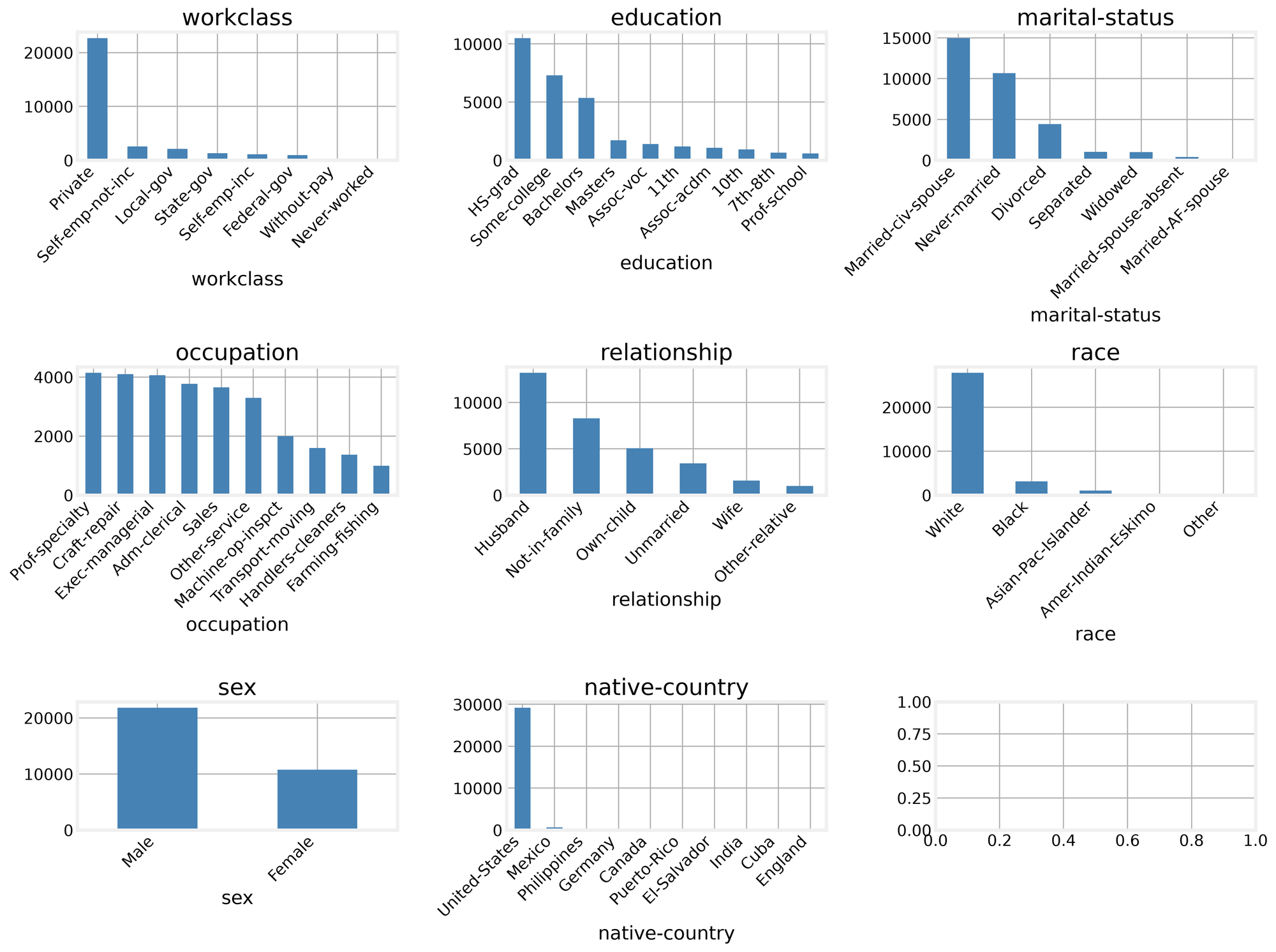
Private sector: 73%, High school: 34%, Married: 56%. The categorical columns show the expected patterns: most people work in the private sector, most have a high school education or some college, and the majority are married.
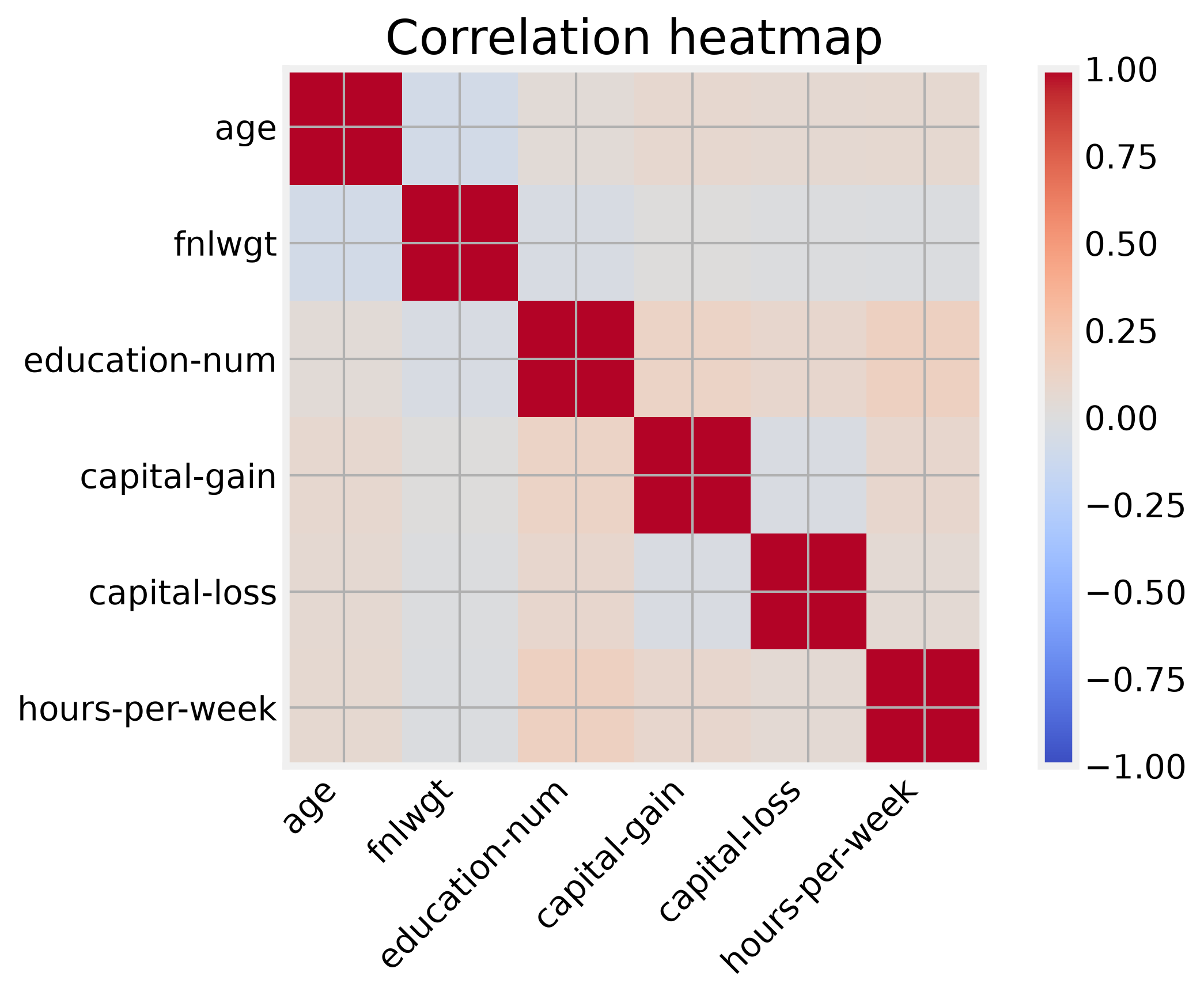
Correlations range from −0.02 to 0.08; age–hours-per-week has the peak at 0.08. The heatmap confirms what the histograms suggested: the numeric features are nearly independent.
Probability language
We start with the fundamental vocabulary. Expectation is the long-run average. For our binary income variable, the expectation equals the probability of high income: 0.2489. Variance measures spread around that expectation. For a Bernoulli random variable, variance equals p(1-p), and our data gives 0.1870—exactly matching the formula.
Covariance measures how two variables move together. The covariance between age and hours-per-week is 15.99, positive but small relative to the scales of the variables. That matches the weak correlation we saw in the heatmap.
Bayes' theorem lets us update probabilities when we have new information. We computed the probability of high income given sex two ways: directly from the conditional mean, and via Bayes' rule using the prior and the likelihood. Both gave 0.3138 for males and 0.1137 for females. The match confirms the theorem works on real data.
Conditional independence asks whether two variables become independent once we condition on a third. We tested whether education and sex are conditionally independent given income. They are not: the joint probability given income differs from the product of the marginals. The difference between the joint probability and the product is 0.045, showing clear dependence. That is expected—education and sex are correlated even within income groups.
The code that computes these quantities is straightforward. The key line for the expectation is a single pandas operation:
p_hat = df_clean['income_binary'].mean() # Expectation of Bernoulli = p
That line gives us 0.2489, the number that will anchor every estimator in the post.