Causal questions and the jobs program data

In Post 13 we learned to ask causal questions, and in Post 14 we saw how randomization answers them cleanly. This post takes the same question into the messy world where we cannot randomize: did a job training program actually raise people's earnings? We will work through the Lalonde NSW data, watch a naive comparison land at $2,071, and then spend the rest of the post earning the right to distrust that number. The through-line is simple. Every method here is a different way of building the same missing thing, a fair comparison group. We will build that missing comparison group three ways, see where they disagree, and ask what that disagreement means for the $2,071.

The dataset is the canonical one for this problem. It comes from Lalonde's 1986 evaluation of the National Supported Work program, and it holds about 2,700 rows across 10 columns. There is a treatment group that went through job training and a control group that did not, plus pre-treatment characteristics, called covariates, like age, education, race, marital status, and earnings in 1974, 1975, and 1978. The experimental subset is small, but the full file carries a large observational control group, which is exactly what makes it a good testbed for comparing designs.

What the data looks like

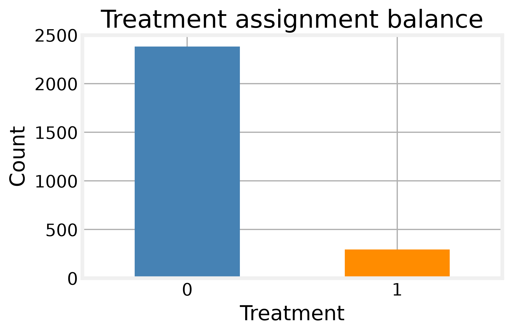
Before any modeling we look at the raw frame. The first thing we check is how common treatment is, because a thin treated arm makes propensity methods harder. We check covariate balance next.

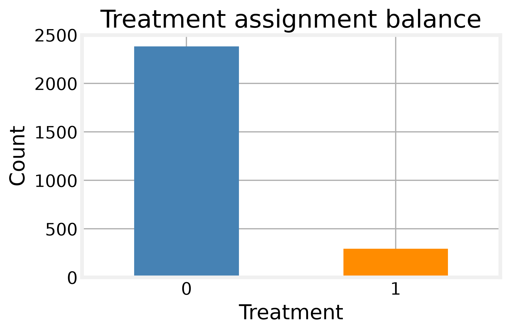
The treatment base rate comes out at 0.110, so roughly one row in nine is treated. That imbalance matters later, because propensity methods have to work harder when one arm is thin. We also find no missing values, and a single duplicate row that we drop, leaving 2,674 rows.

The summary statistics confirm the same imbalance and add the shape of the earnings distribution.

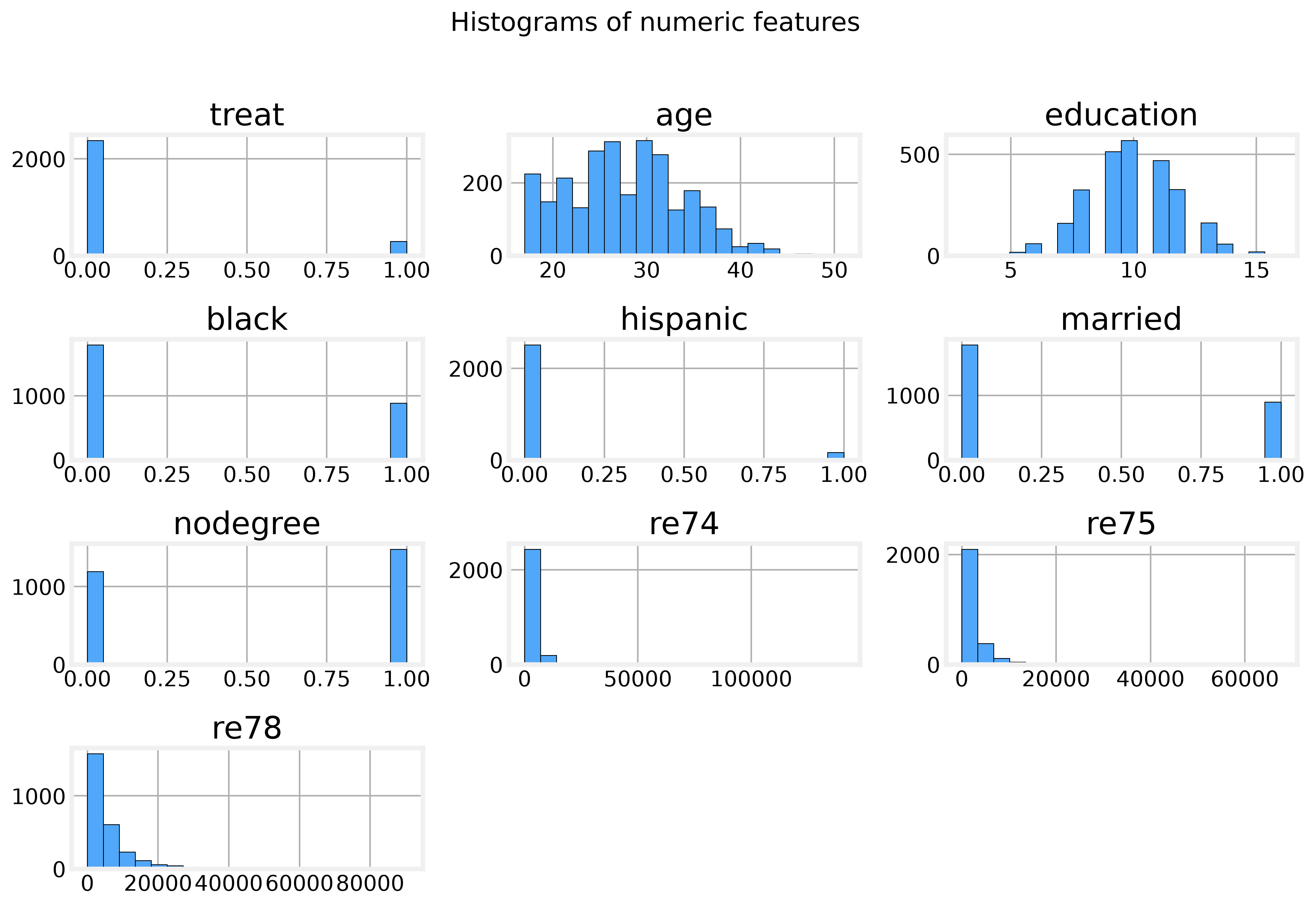
Earnings in 1974, 1975, and 1978 are heavily right-skewed with many zeros, and the outlier counts are large: 157 in re74, 172 in re75, and 146 in re78. The categorical features are binary, and black and hispanic are correlated with treatment assignment. The correlation heatmap shows re74, re75, and re78 moving together, which is expected since they measure earnings over time. The practical consequence is that treated and control units differ on age, education, race, marital status, and prior earnings, so confounding is likely and we will need to adjust for it. We keep re74 and re75 as pre-treatment covariates and leave re78 out of the feature set, because it is the outcome.

Foundations

The imbalance above is confounding. Here are the definitions we need to name it. Randomized controlled trials are the gold standard because random assignment makes treatment independent of potential outcomes. Potential outcomes are the outcomes a unit would have under each treatment, and the causal effect is the difference between them. Counterfactuals are the potential outcomes we never observe, and confounding is what happens when a variable drives both treatment and outcome, creating an association that is not causal.

We can measure the damage directly. The naive difference in means between treated and control on 1978 earnings is $2,071.01. That number is not the effect of the program. It is the effect of the program plus every way the two groups already differed. Standardized mean differences compare covariate means in standard-deviation units; values above about 0.1 signal imbalance. The standardized mean differences confirm the imbalance: black sits at 1.381, married at -0.390, age at -0.328, and re75 at -0.301. Anything above about 0.1 is a warning, and these are far past it.

Graphs for causality

The imbalance above suggests confounding. To decide which variables to adjust for, we use causal DAGs, which encode our assumptions about how the data was generated. The backdoor criterion then tells us which variables to adjust for so that the remaining association is causal. The do-calculus rewrites causal expressions built with the do-operator, which sets a variable by intervention, into ordinary probabilities we can estimate from data. The payoff is easiest to see on a small simulation where we know the truth.