Forecasting household power use

In Post 14 we built the baselines that every forecast has to beat, and in Post 13 we learned to read autocorrelation and lag features. Now we point both at a real meter. This post takes four years of minute-by-minute household electricity readings and turns them into a working forecast of daily power use, ending with a seasonal ARIMA that lands at 0.2774 kW (kilowatts) mean absolute error against a seasonal naive baseline of 0.2929 kW. That is a small win, and the size of the win is the story. The through-line for the whole post is the meter itself: one device, one column, and a chain of decisions about what we are allowed to feed a model that has to predict the future from the past.

We resample the raw readings into hourly and daily series, define smoothing and detrending baselines, formalize stationarity with the augmented Dickey-Fuller test, fit the ARIMA family plus a state space model, model volatility with GARCH, test lead-lag with Granger causality, backtest with rolling windows, and preview two deep forecasters. The dataset is the University of California, Irvine (UCI) Individual household electric power consumption record, and the target is the hourly mean of Global_active_power in kilowatts.

The meter and its gaps

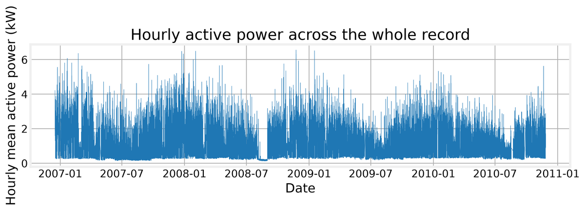
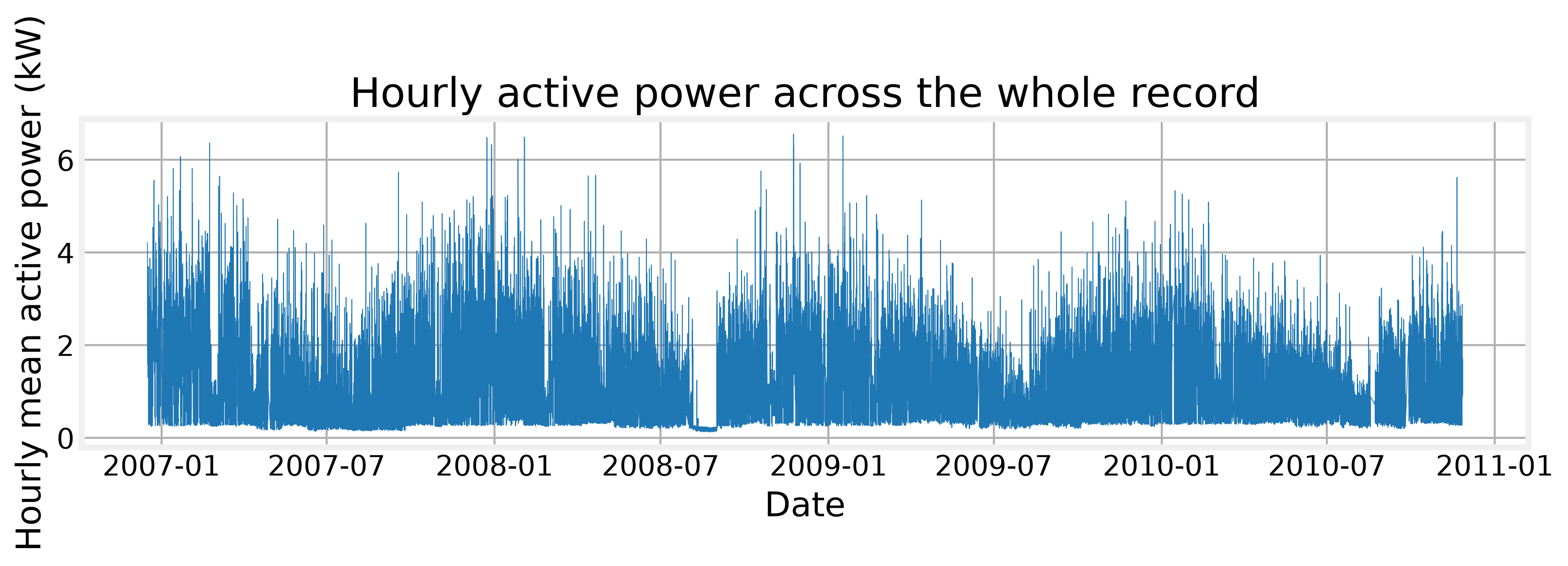
The file is a semicolon-separated text dump of about 130 MB on disk, a little over two million minute-level rows and seven measured columns, running from 2006-12-16 to 2010-11-26. Before any modeling we asked four questions of it: what is in the file, what is missing, what does the target look like, and which columns would leak the future. The first answer is that every one of the seven columns is missing exactly 25,979 minutes, 1.252 percent of the record, and the gaps come in short runs. We resample to hourly means, interpolate runs of up to three hours, and drop the rest. That leaves 34,190 clean hours out of 34,589 expected timestamps, so we lose 399 hours and keep a regular index that SARIMAX requires.

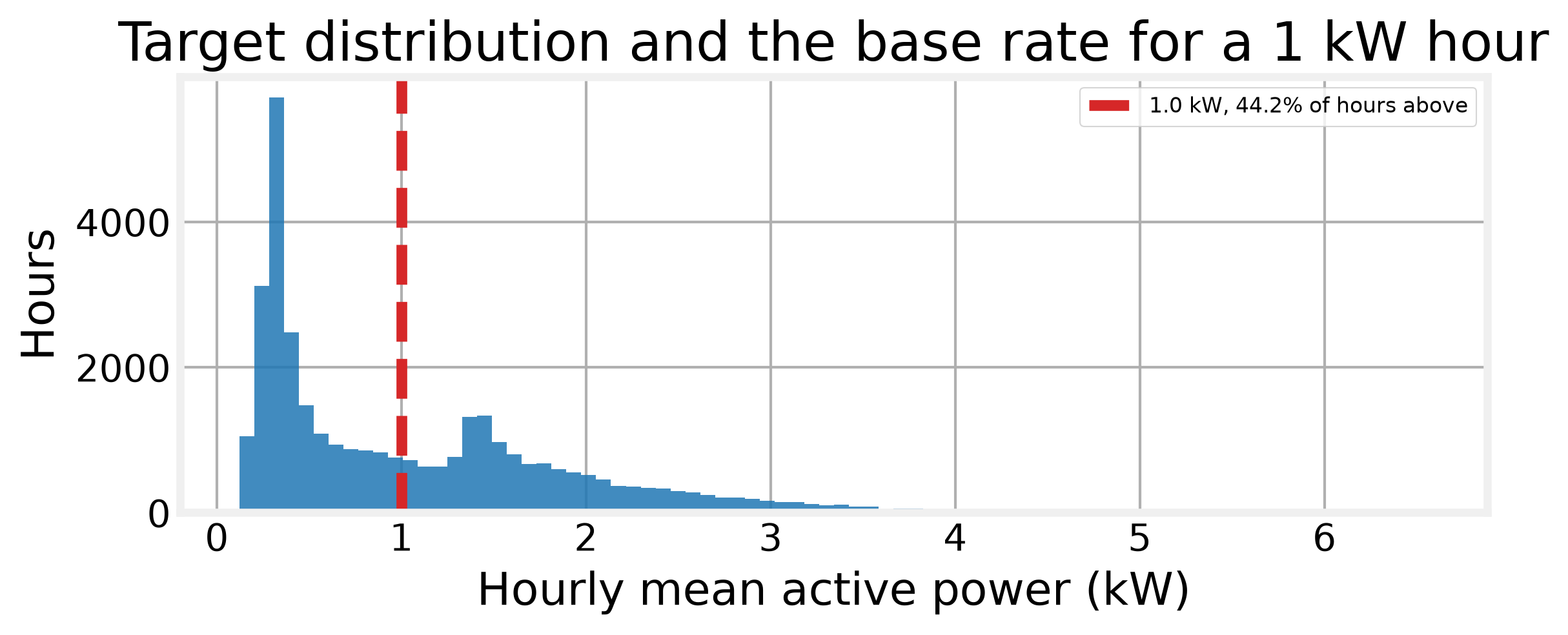
The target is right skewed, meaning a long tail of high values pulls the mean above the median. The median hourly reading is 0.803 kW while the mean is 1.092 kW, and 44.15 percent of hours sit above the 1 kW mark. That base rate is the floor any hit-rate claim has to clear, and it is worth remembering when a model looks impressive.

The leakage question is the one that decides the rest of the notebook. Global_reactive_power, Voltage and Sub_metering_3 all correlate with the target, at 0.312, -0.379 and 0.696 respectively, but every one of them is recorded in the same minute as the target. None is known ahead of the forecast origin, and the sub-meter is a component of the total by construction. They stay out of every forecast input. We only use them later to show lead-lag structure, never as a predictor.

To see the seasonal shape, we plotted the average day and week.

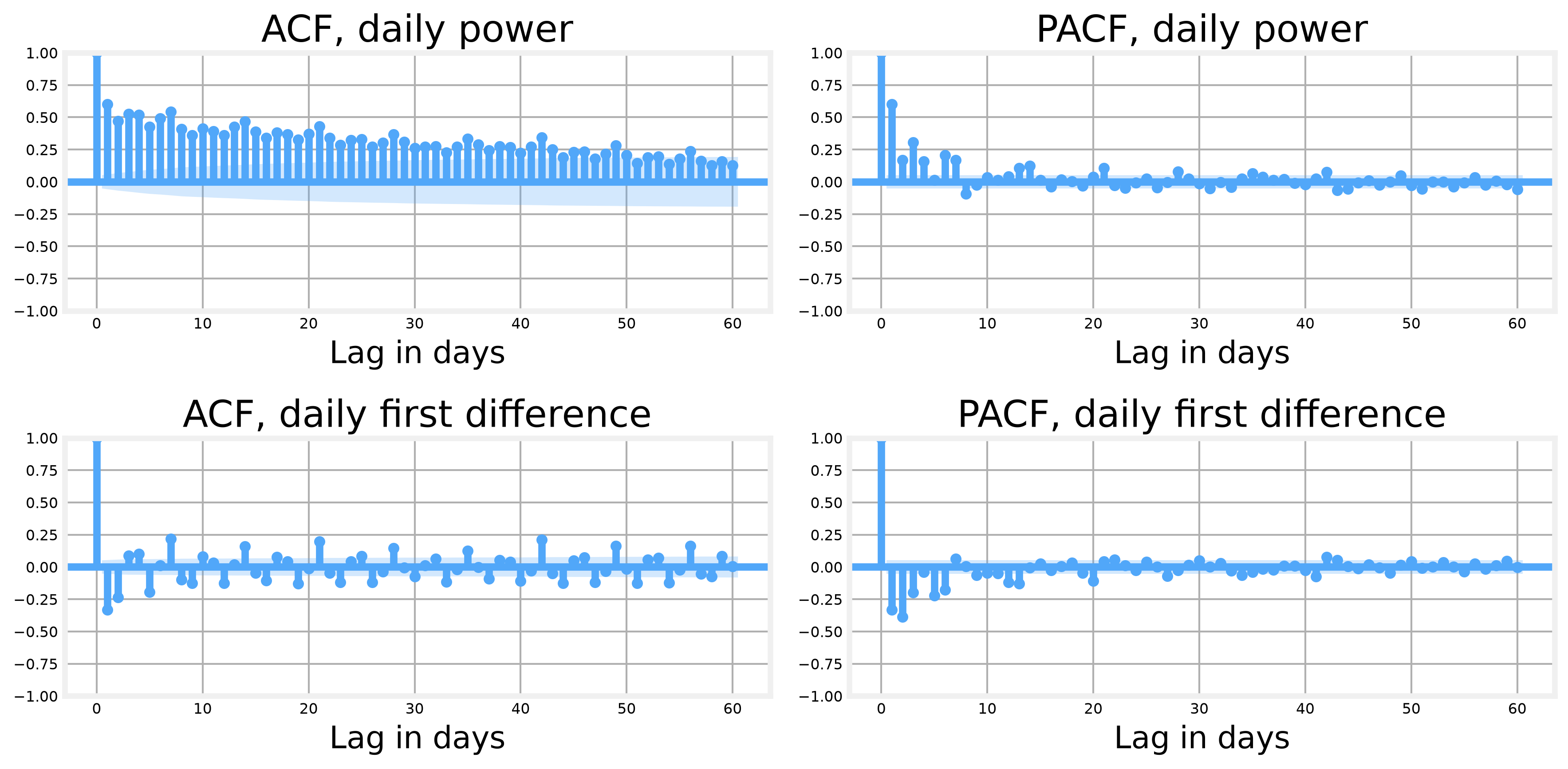
The daily profile has a morning rise and a heavier evening peak, and the weekly profile is flatter at the weekend. That tells us the daily series wants a seasonal period of 7 and the hourly series wants 24. Autocorrelation is the correlation of a series with its own past values. Partial autocorrelation removes indirect paths through shorter lags to show the direct link at each lag. A unit root means shocks persist and one difference usually makes the series stationary. The autocorrelation of the raw daily series decays slowly and stays positive far past 60 days, the signature of a unit root, so we difference before fitting an ARMA structure. The partial autocorrelation of the first difference cuts off after the first couple of lags, so a low-order AR term is enough.

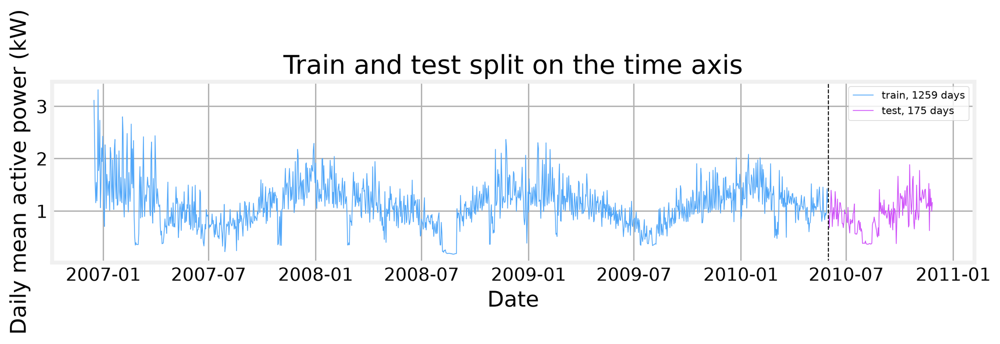
We hold out the last 180 days as a test window, which gives 1,259 training days and 175 test days after the split at 2010-05-31. The level drifts across the record, so a single fixed split would flatter any model, and the backtests later have to roll forward.

Smoothing starters

With the split fixed, the simplest thing to try is a weighted average of the past. Exponential smoothing has one parameter, alpha, that decides how fast the past fades. Holt-Winters adds a trend term and a repeating seasonal term, so a series with a weekly cycle gets a weekly shape instead of a flat level. Differencing subtracts a lagged copy of the series to remove a trend or a season, and detrending removes a smooth trend, here a centered rolling mean, without touching the shape of the cycle.

With the split fixed, the first baseline is a weighted average of the past; the wrapper below fits both a flat level and a weekly seasonal shape.

def fit_ets(train, horizon, trend=None, seasonal=None, season_len=None):
    # One wrapper for plain exponential smoothing and for Holt-Winters.
    model = ExponentialSmoothing(train, trend=trend, seasonal=seasonal,
                                 seasonal_periods=season_len,
                                 initialization_method='estimated')
    return np.asarray(model.fit().forecast(horizon), dtype=float)

Scored on the same 180-day window, the seasonal naive baseline lands at 0.2929 kW, simple exponential smoothing at 0.2848 kW, and Holt-Winters at 0.2779 kW. Holt-Winters wins because a flat level cannot follow a weekly cycle, and both beat the naive line rather than zero, and beating the seasonal naive baseline is the test.