Flows and diffusion models on digits

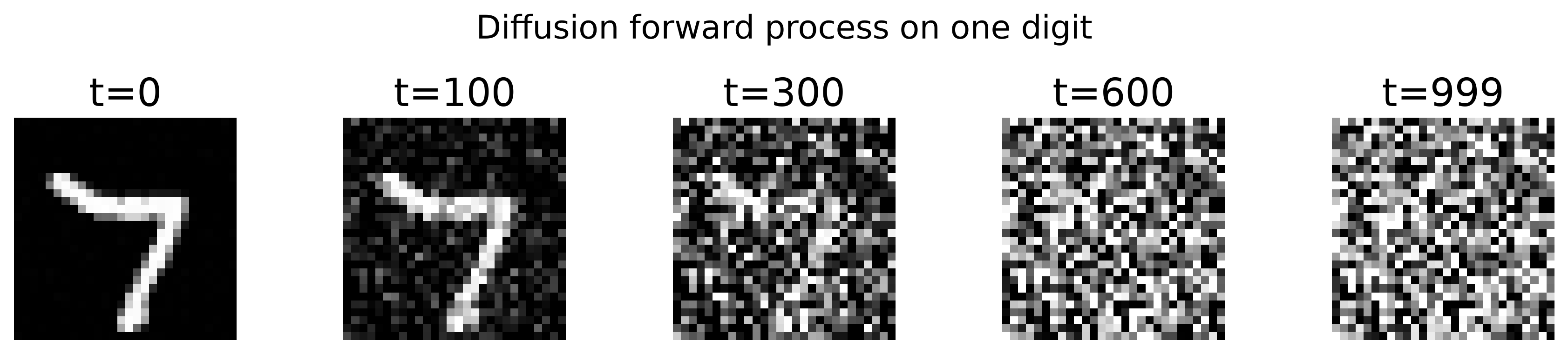
In Post 32 we built the machinery of generative modeling: latent variables, likelihoods, and the idea that a model can learn a distribution rather than a label. This post puts that machinery to work on MNIST. We train an exact-likelihood RealNVP flow, then a small DDPM diffusion model, and sample from the second with DDIM in 25 steps. The flow beats a Gaussian baseline by 105.6 nats per image, where a nat is the natural-log unit of information and lower negative log-likelihood is better. The diffusion model, trained for three epochs on 6000 digits, produces recognizable samples in 0.007 seconds. The through-line for the whole post is a single idea: a generative model is a machine for turning noise into structure, and the two families we build here disagree about which direction to run that machine.

The dataset is MNIST, 70,000 grayscale images at 28 by 28 pixels, downloaded through torchvision. Digits are small, fast on a laptop, and still show every behavior we care about. We work on a 6000-image training subset and a 1000-image test subset, both drawn with seed 42, because the full set is unnecessary for a run that finishes in minutes.

What the digits tell us

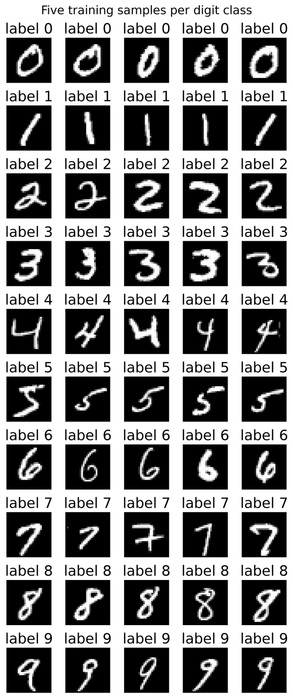
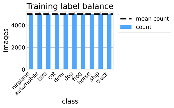
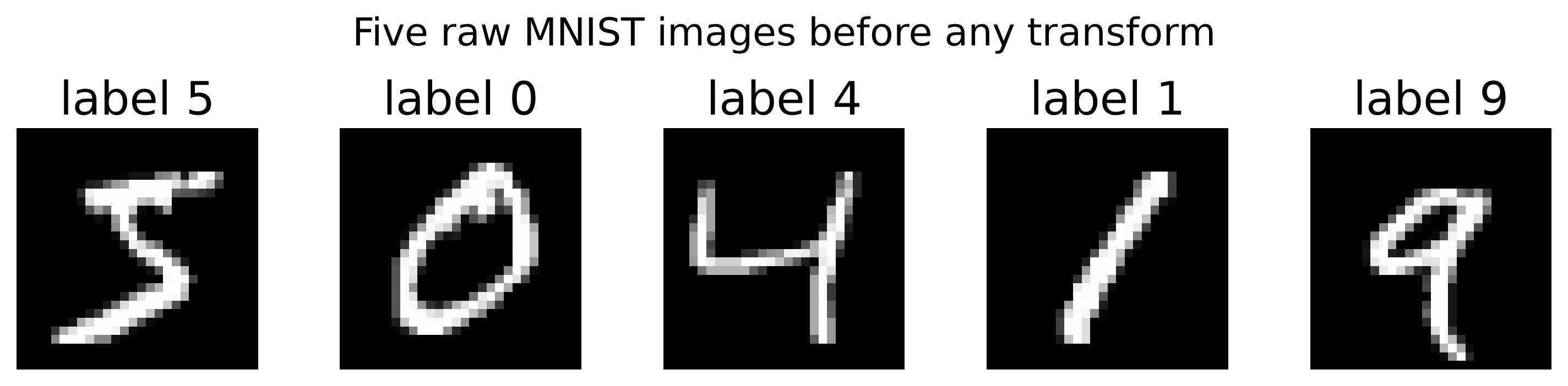
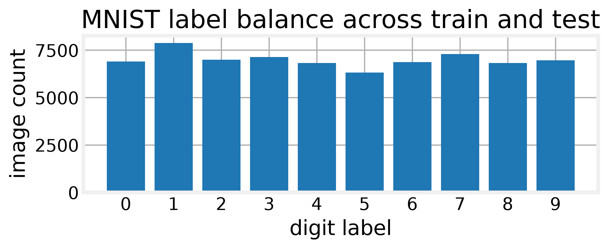
Before training anything we look at the raw images and the metadata. The label counts run from 6313 for the digit 5 up to 7877 for the digit 1, and the most frequent class sits at a base rate of 0.1125, close enough to uniform that a random subset keeps every class. The metadata has zero missing values, and the first hundred training images contain no NaN pixels, so nothing needs imputation. Every image is 28 by 28 with a single channel, which lets the models use fixed convolutional shapes. Here are five of them:

The pixel intensity histogram is the finding that shapes the modeling. MNIST is mostly black background with a bright stroke, so the distribution is heavily skewed toward zero. That skew is why we rescale pixels to the range from -1 to 1 before feeding them to a flow, and why the noise we add during diffusion has to be scaled to match.

We also check for duplicates and train/test leakage, where leakage means a test image that also appears in training. There are zero duplicate training images and zero leakage candidates, so the 1,000 held-out test images stay clean. The lowest-contrast digits have a pixel standard deviation of 41.9 on the original 0–255 scale, before the rescaling, and those are the visually hardest cases, which is why we judge those cases on the sample grid rather than the loss.

Exact likelihoods

That rescaling hands the flow a distribution on -1 to 1 that is still overwhelmingly dark, and the flow's job is to bend it into something we can sample from. A normalizing flow learns an invertible map from data to a simple base density. The exact likelihood is log p(x) = log p(z) + log |det J|, where J is the Jacobian of the map. RealNVP builds that map from coupling layers, each of which splits the image by a checkerboard mask, transforms one half conditioned on the other, and leaves the log-determinant cheap to compute. The same invertibility idea has cousins that give up the exact determinant for something else. Glow adds invertible 1x1 convolutions on top. PixelCNN models pixels autoregressively, meaning it predicts pixel n from pixels 1 to n−1. Energy-based models define an unnormalized energy, a score that ranks images by plausibility but isn't scaled to sum to one, and they need sampling to train or generate.

The coupling layer is the whole trick, so it is worth seeing in full. The mask splits the image, a small convolutional network predicts a scale and a shift from the masked half, and the unmasked half is transformed by those. The log-determinant is just the sum of the scale over the transformed pixels.

def forward(self, x):
    x1 = x * self.mask
    st = self.net(x1)
    s = torch.tanh(st[:, 0:1]) * 2.0
    t = st[:, 1:2]
    x2 = x * (1.0 - self.mask)
    y = x1 + (1.0 - self.mask) * (x2 * torch.exp(s) + t)
    logdet = (s * (1.0 - self.mask)).sum(dim=[1, 2, 3])  # exact log-determinant
    return y, logdet

We stack six of these layers with alternating masks and train for three epochs. The training NLL swings hard between epochs, from 572.4 nats per image in epoch 1 to -305.5 in epoch 2 and -350.4 in epoch 3, which is mostly an artifact of initialization: an untrained scale head makes epoch 1 a measure of where we started, not of the model. On the test set the numbers are the ones that matter: a plain Gaussian baseline gives 1083.1 nats per image, and RealNVP gives 977.5. The flow improves on the baseline by 105.6 nats. That gap is the whole lesson of exact likelihoods: the model is measurably better than noise, and we can say so in a single number.