Clustering and Anomaly Detection on Handwritten Digits

In the previous posts we built classifiers that needed labels for every image, but most data arrives without a teacher. This post turns that assumption on its head: we hand 70,000 handwritten digits to a collection of unsupervised algorithms and ask them to find structure on their own. By the end we reach an anomaly detector that separates odd digits from a clean reference family with an AUROC of 0.967 (the area under the receiver operating characteristic curve, or the probability that a random odd digit scores more anomalous than a random clean digit), and along the way we learn why some clustering methods see digit classes while others see only style pockets. The through-line for this whole exploration is a simple question: when no one tells the algorithm what a seven looks like, what does it discover anyway?

We work with MNIST, the 70,000 grayscale digits that have powered machine learning research for decades. Each image is 28 by 28 pixels, and the ten digit classes are balanced enough that chance performance sits near zero for our clustering metrics. We load the full dataset through torchvision, combine train and test splits into one array of 70,000 images, and keep a small metadata table with the true labels and source split. Those labels stay out of the clustering algorithms entirely; we use them only to score how well unsupervised structure matches human categories.

Looking at the data first

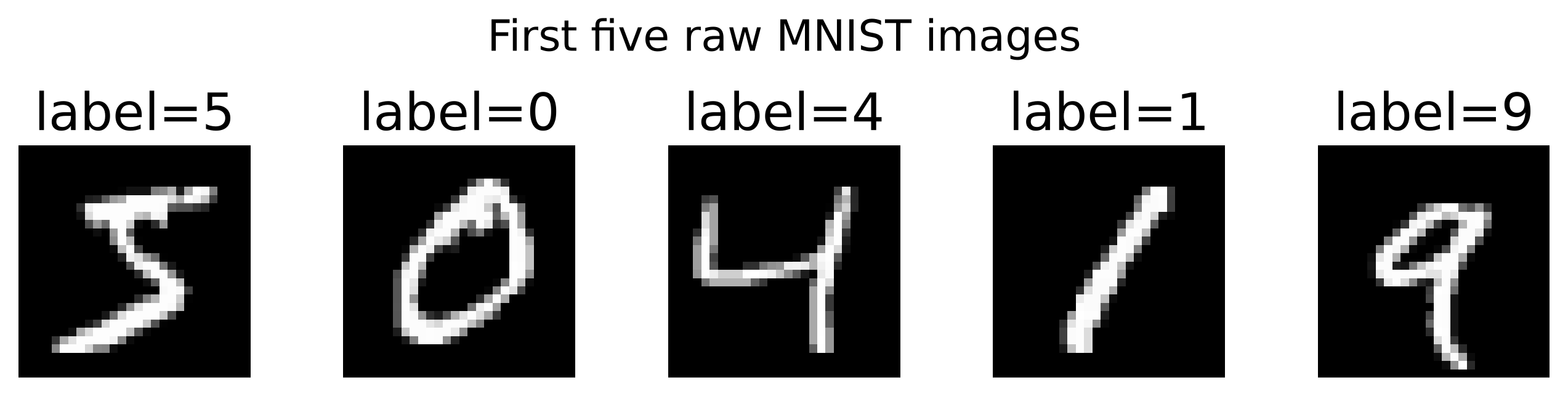
Before any clustering runs, we inspect what we are working with. The raw images confirm what we expect: clean black backgrounds, white ink strokes, and clear visual differences between digits.

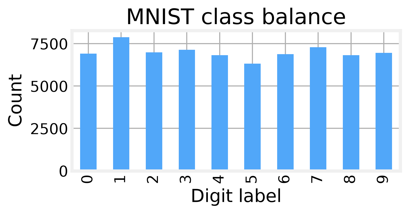
The class balance plot shows why ten clusters is a natural starting point. The largest digit class, the digit 1, accounts for only 11.25 percent of the data, so no single group dominates.

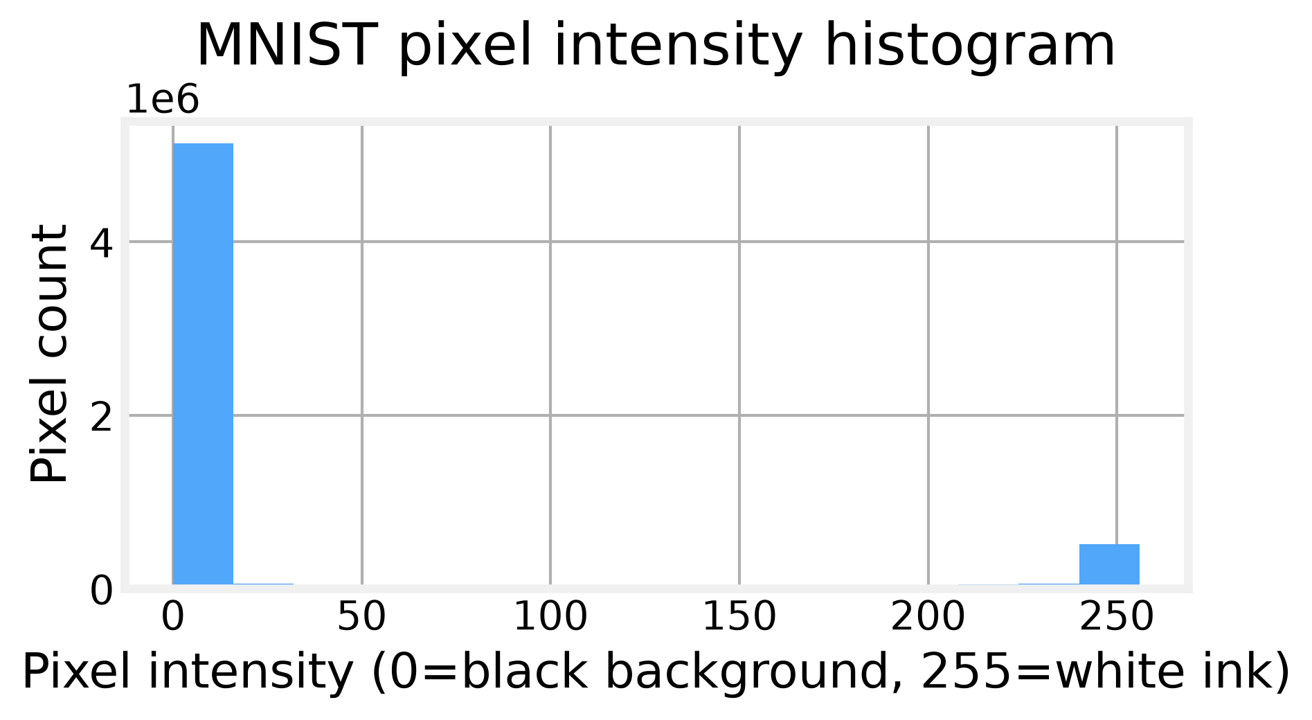
We scan for missing values and find none, and a hash-based duplicate check confirms zero exact overlaps between train and test. The pixel intensity histogram reveals that background pixels dominate, with a long tail of ink strokes at higher intensities.

A few images stand out as genuinely odd. The densest images in the dataset, measured by the fraction of pixels above the 128 threshold, are so heavily inked that they could pass for another digit entirely.

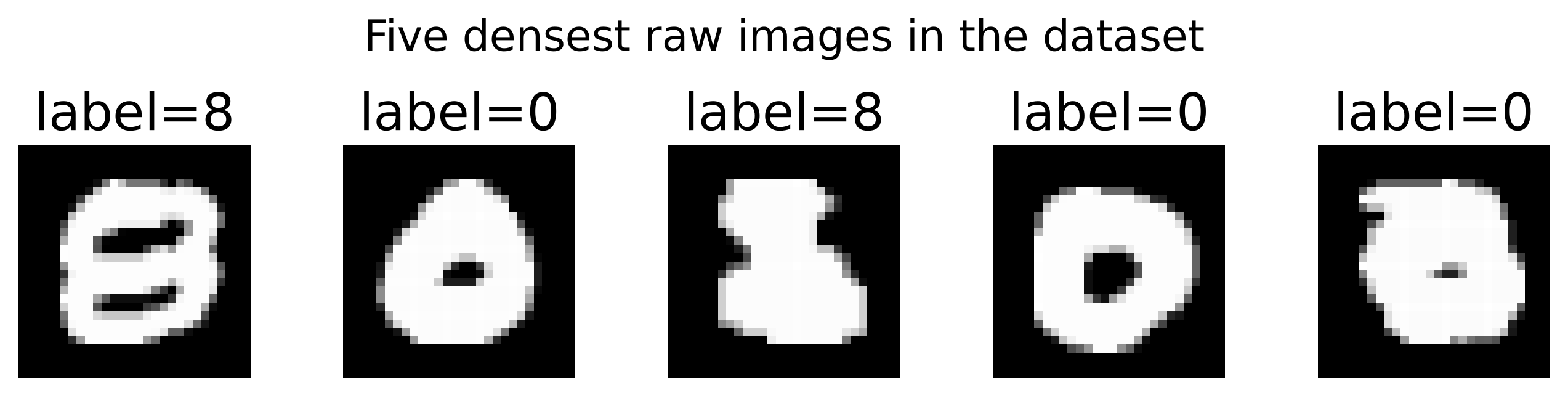
These findings drive every choice that follows. Balanced classes make ten the default cluster count. The absence of duplicates lets us sample freely across splits. And those dense confusable images give anomaly detection a natural test case later.

Flat clusters

The first assumption is that each digit class occupies one smooth blob in pixel space, so we start with k-means. k-means partitions the images into k groups by learning centers that are averages in pixel space. Lloyd's algorithm iterates between assigning each image to its closest center and recomputing the centers from the current assignment. k-means++ handles the initialization by spreading the starting centers so no two begin too close together.

We work on a fixed subset of 5000 images, one per digit class, to keep every method within a reasonable runtime. A principal component analysis (PCA) projection to 50 components retains 82.6 percent of the variance and removes pixel noise that would otherwise dominate distance calculations. For a baseline we run k-means with ten centers on the PCA features and read the ARI and NMI from the resulting labels.

# k-means baseline: 10 centers, k-means++ init, Lloyd updates
kmeans = KMeans(n_clusters=10, init="k-means++", n_init=10, random_state=SEED)
km_labels = kmeans.fit_predict(X_pca_cluster)
km_ari = adjusted_rand_score(y_cluster, km_labels)

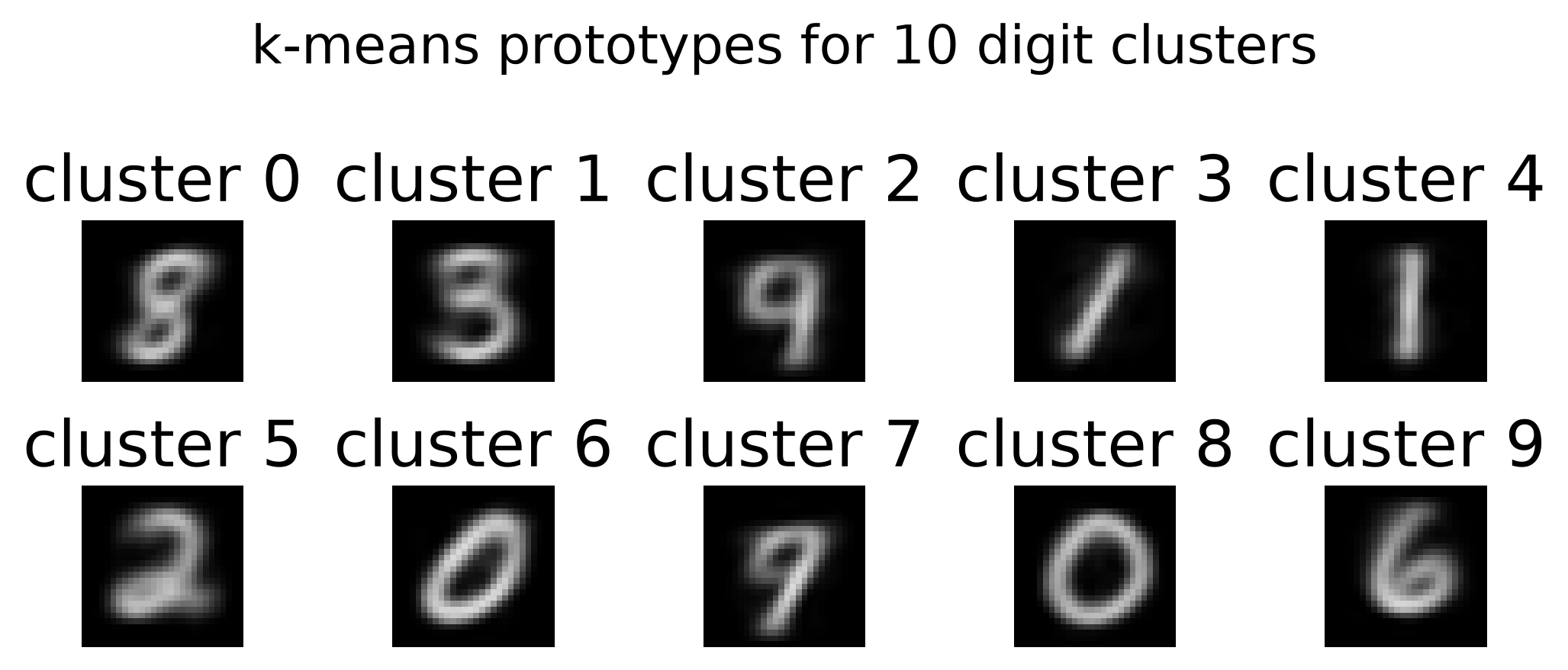
The adjusted Rand index (ARI) counts whether pairs of images stay together or apart across the true labels and the predicted clusters; normalized mutual information (NMI) measures how much the predicted clusters reduce uncertainty about the digit labels. The resulting prototypes, mapped back from PCA space to pixels, look like digit classes. The adjusted Rand index lands at 0.350 and the normalized mutual information at 0.488, both far above the chance values implied by balanced classes.

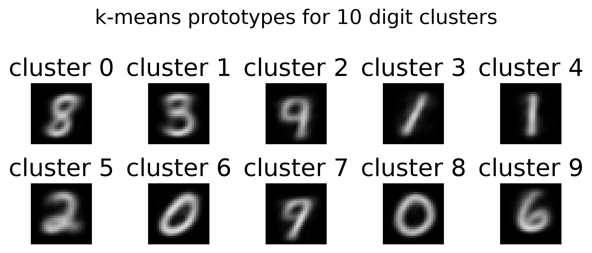
The prototypes are readable, but visually related classes like 3, 8, and 9 can share a fuzzy center. That is the linear centroid limit, and it is exactly the problem mixture models address later.