Stochastic Blog

Information Theory in One Sitting

In Posts 3 and 4 we built the probabilistic foundations and learned how to update beliefs with Bayes' rule. Now we put that machinery to work on a concrete question: how much information is actually in a piece of text? This post measures that quantity on WikiText-2, a two-million-token slice of Wikipedia, and ends with a number that quantifies how predictable English really is. By the time we finish, we will have watched the cost of encoding a token fall from 15.99 bits under a uniform guess to 8.39 bits with a bigram model, and we will understand every step between those two extremes. A token is one lowercase word here, and a bigram model predicts each token from the previous token alone.

The through-line of this post is a simple one: information is a budget. Every token in a text costs bits to transmit, and the whole game of language modeling is spending fewer bits than a naive encoding would. We start with the cheapest possible accounting, the entropy of a single token, and work our way up to the conditional models that actually predict words. Along the way we meet the tools that connect raw counts to real predictions: cross-entropy, KL divergence, Jensen-Shannon divergence, and mutual information. Each one tightens our accounting by a different mechanism, and each one pays off when we finally measure bits per token on held-out data.

The Data

WikiText-2 comes from Hugging Face with train, validation, and test splits already separated, which is exactly what we need for honest evaluation. The train split holds 36,718 documents and about 1.76 million tokens after a simple lowercase word tokenizer. The validation and test splits are smaller, 184,069 and 207,136 tokens respectively, and they share no documents with the training set. That clean separation matters: when we measure a model on validation, we are measuring generalization, not memorization.

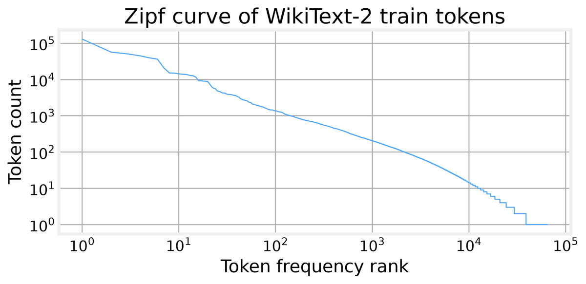
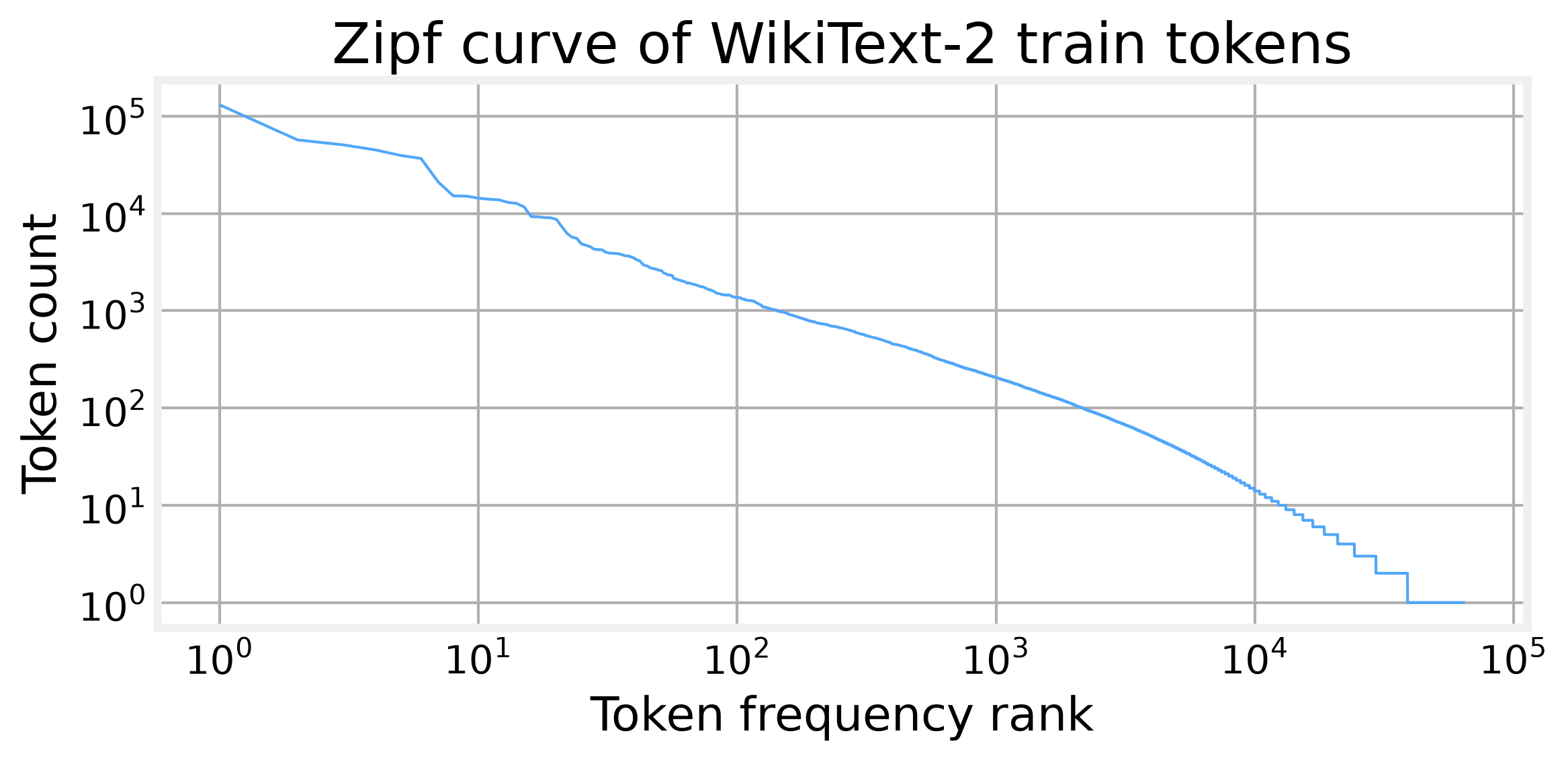
Plotting token frequency against rank on log-log axes produces a nearly straight line, the classic Zipf curve. A handful of tokens dominate: the most common token, "the", appears with probability 0.0744, meaning it accounts for roughly one token in thirteen. The vocabulary is large, 64,916 distinct tokens, but the distribution over it is anything but uniform. That skew is the first hint that information is cheaper than a naive count would suggest.

The Zipf curve of WikiText-2 train tokens shows a nearly straight line on log-log axes, the signature of a heavily skewed frequency distribution.

The second finding is more practical. When we check the validation split against the training vocabulary, we find a substantial out-of-vocabulary rate. A fixed-vocabulary model needs an <unk> token to absorb those unseen words, and it needs smoothing to keep every probability nonzero.

Entropy

The OOV problem is about tokens the model has not counted. Entropy is the baseline for the tokens it has counted. Entropy is the first topic, and it answers the simplest version of our budget question: how many bits does one token cost on average? For a uniform distribution over V tokens, the answer is log2 V bits. With 64,917 tokens in our closed vocabulary (the fixed list of tokens the model can emit), that baseline sits at 15.9863 bits per token. But our distribution is not uniform, and the Zipf curve tells us why.

The empirical entropy of the training tokens comes to 10.9438 bits per token. The skew of the frequency distribution saves us 5.04 bits compared to a fair draw from the whole vocabulary. That is the first payoff of the Zipf curve: a few frequent tokens make token prediction easier than a uniform guess would suggest. The dominant token's share buys much of that saving, while the long tail of rare words contributes less to the average cost than their sheer number might imply.

def empirical_entropy(counts):
    # Average surprise of one token under the observed distribution.
    total = sum(counts.values())
    return -sum((count / total) * math.log2(count / total) for count in counts.values() if count > 0)

The entropy calculation is a sum over all tokens of probability times log probability, negated. It is the average number of bits a perfect encoder would spend per token, and it is the floor that no model can beat. Everything we do from here on is an attempt to approach that floor with a model that does not know the true distribution.

Cross-Entropy

Cross-entropy is the second topic, and it measures what happens when we use the wrong distribution to encode the right one. The formula is the same shape as entropy, but the log probability comes from a model Q while the averaging happens under the data distribution P. If Q assigns zero probability to any token P can produce, the cost is infinite.

That is exactly what happens when we try to encode the training distribution using the raw validation counts. The validation split does not contain every training token, so the naive cross-entropy comes back as infinity. The fix is add-one smoothing, which gives every vocabulary token a small probability floor. With smoothing, the cross-entropy between train and validation lands at 11.3583 bits per token.

def laplace_probs(counts, vocab, alpha=1.0):
    # Add-one smoothing keeps every vocabulary token reachable, so cross-entropy stays finite.
    total = sum(counts.values())
    return np.array([(counts.get(token, 0) + alpha) / (total + alpha * len(vocab)) for token in vocab], dtype=float)

The smoothed number is close to the train entropy of 10.94 bits, which tells us the two distributions are similar. But cross-entropy is not symmetric, and the direction of the comparison matters. That asymmetry is the subject of the next topic.

KL Divergence

KL divergence is the third topic, and it isolates the extra cost of using the wrong distribution. It is defined as the cross-entropy minus the entropy of the true distribution, which leaves only the penalty for the mismatch. When the two distributions are identical, the penalty is zero. When they differ, it is positive, and it is not symmetric.

We compute it in both directions on our data. From train to validation, the KL divergence is 0.4145 bits per token. From validation to train, it is 0.9607 bits per token. The asymmetry gap is 0.5462 bits, and it is not an accident. The training distribution has more mass on rare tokens, so encoding validation under train costs less than the reverse. The direction with the larger penalty is the one where the model distribution has holes that the data distribution fills.

This function computes the two numbers above:

def kl_divergence(p_counts, q_counts, vocab, alpha=1.0):
    p_probs = empirical_probs(p_counts, vocab)
    q_probs = laplace_probs(q_counts, vocab, alpha=alpha)
    return cross_entropy(p_probs, q_probs) - empirical_entropy(p_counts)

It returns 0.4145 and 0.9607 bits per token in the two directions. KL divergence is the workhorse of many machine learning methods, but its asymmetry can be awkward when we want a single number for how far apart two distributions are. That is the gap the next topic fills.

Jensen-Shannon

Jensen-Shannon divergence is the fourth topic, and it solves the symmetry problem by comparing both distributions to their midpoint. Define M as the average of P and Q, then JSD is the average of the two KL divergences from P and Q to M. The result is symmetric, always finite, and bounded above by 1 bit.

On our data, the JSD between train and validation token distributions is 0.1247 bits. That is a small number, confirming that the two splits are close despite the rare-token differences that made the naive cross-entropy infinite. The symmetry is built into the definition, so swapping the arguments changes nothing. This makes JSD the right tool when we want a single, stable measure of distribution distance.

def js_divergence(p_counts, q_counts, vocab):
    p = empirical_probs(p_counts, vocab)
    q = empirical_probs(q_counts, vocab)
    m = 0.5 * (p + q)
    # Average the KL divergences from each distribution to the midpoint.
    return 0.5 * kl_between(p, m) + 0.5 * kl_between(q, m)

The JSD tells us the splits are consistent, which is reassuring. But it does not tell us anything about the structure within the text. For that, we need to look at pairs of tokens, not single ones.

Mutual Information

Mutual information is the fifth topic, and it asks a different question: how much does knowing the current token reduce uncertainty about the next one? This is the signal that any sequential model exploits, and we can measure it directly from bigram counts.

We restrict the vocabulary to the 5,000 most frequent tokens plus <unk>, which covers 84.1 percent of the training tokens. That reduction keeps the bigram table manageable: 339,290 distinct bigrams instead of the billions we would get with the full vocabulary. The mutual information between adjacent tokens comes to 2.2641 bits.

The loop that sums those terms is:

mutual_info = 0.0
for (x, y), count in train_bigram_counts.items():
    p_xy = count / xy_total
    p_x = x_marginal[x] / xy_total
    p_y = y_marginal[y] / xy_total
    # Positive MI means the pair is more common than chance would predict.
    mutual_info += p_xy * math.log2(p_xy / (p_x * p_y))

Two and a quarter bits is a real signal, but it is a fraction of the 10.94 bits of entropy per token. Knowing the previous word saves us about a fifth of the cost of guessing the next one. That is the budget the bigram model will spend, and the next section shows exactly what it buys.

Bits per Token

Bits per token is the sixth topic, and it is the number that actually matters for language modeling. It is the average negative log2 probability a model assigns to each token, and lower is better. Perplexity is just 2 raised to that number, so 8.39 bits per token corresponds to a perplexity of 335.39.

We evaluate two models on the validation split. The first is a Laplace-smoothed unigram model, which ignores context entirely and assigns each token its smoothed marginal probability. It scores 8.4392 bits per token. The second is a smoothed bigram model, which conditions each token on the previous one. It scores 8.3897 bits per token. The bigram saves 0.0495 bits per token on validation, and the same pattern holds on the test split, where the saving is 0.0435 bits.

The scorer that produced these numbers is:

def bigram_bits_per_token(docs, unigram_counts, bigram_counts, vocab, alpha=1.0):
    # First token uses the unigram fallback, later tokens use a smoothed bigram model.
    denom = sum(unigram_counts.values()) + alpha * len(vocab)
    logprob_sum = 0.0
    token_count = 0
    for doc in docs:
        if not doc:
            continue
        logprob_sum += math.log2((unigram_counts.get(doc[0], 0) + alpha) / denom)
        token_count += 1
        for prev, curr in zip(doc, doc[1:]):
            context_count = unigram_counts.get(prev, 0)
            joint_count = bigram_counts.get((prev, curr), 0)
            prob = (joint_count + alpha) / (context_count + alpha * len(vocab))
            logprob_sum += math.log2(prob)
            token_count += 1
    return -logprob_sum / token_count

The saving is small, only about five hundredths of a bit, but it is real and it reproduces on held-out data. That gap is the practical payoff of the mutual information we measured. The remaining 8.39 bits are the irreducible difficulty of word prediction, the cost of the world's unpredictability that no amount of local context can remove.

Closing

We started with a uniform distribution costing 15.99 bits per token and ended with a bigram model spending 8.39 bits. The Zipf curve explained the first drop, from uniform to empirical entropy. Smoothing kept our calculations finite when the validation split revealed tokens the training set never saw. JSD confirmed the splits were close, and mutual information quantified the signal between adjacent words. The bigram model turned that signal into a measured, reproducible saving on both validation and test.

The notebook simplifies a great deal. Our tokenizer is a lowercase word splitter, not a subword tokenizer, and our vocabulary is capped at 5,000 words plus an unknown token. A production language model would use byte-pair encoding, a much larger vocabulary, and a neural architecture that conditions on far more than one previous token. The smoothing is add-one, which is crude; modern models use learned embeddings and softmax over the full vocabulary. What survives all those simplifications is the accounting: every model is spending bits, and the tools we built measure exactly how well it spends them.

Post 6 starts where this one stops. It replaces the smoothed bigram counts with a small neural language model and watches the bits per token fall. The question it answers is the one we leave open here: how much of the remaining 8.39 bits can a model that conditions on a longer context recover?

Exercises

Try the exercises in the notebook to deepen the feel for these quantities. Remove the 100 most frequent tokens and watch entropy rise. Drop the smoothing parameter from 1.0 to 0.1 and see how cross-entropy and bits per token shift. Swap train and validation in the JSD and confirm it stays symmetric. Compute mutual information on character-level bigrams instead of word-level bigrams. And if you are feeling ambitious, implement a trigram model with smoothing and report its bits per token.