Bandits on movie ratings

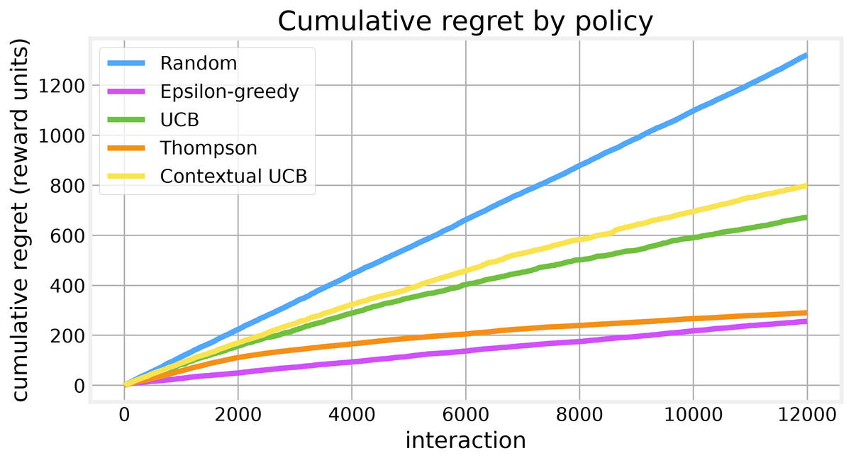
In the background posts we built the pieces of a recommender: a way to score movies, a way to split users, and a way to measure whether a prediction was any good. This post turns the problem around. Instead of predicting a rating and checking it later, we recommend one movie at a time and learn from the answer we get back. Over 12,000 interactions with 12 popular movies, a plain epsilon-greedy policy reaches a mean high-rating rate of 0.8826, against 0.7905 for a policy that guesses at random. That gap is the lesson: how we choose what to show matters, not only how accurately we predict ratings.
Think of the recommender as a row of slot machines, one per movie, each with an unknown payout. Every pull costs a recommendation, and we only ever see the payout of the machine we pulled. The job is to spend our pulls well, pulling the good machines often while still spending enough on the rest to be sure they are not secretly better. That is the bandit framing, and we will carry it through every policy below.
We work with MovieLens 1M, the same ratings file from earlier posts: 1,000,209 ratings across 6,040 users and 3,883 movies. We download it, check the schema, and confirm there are no missing values in the three raw files. From there we build the reward, the arms, and the contexts, then replay five policies against a fixed ground truth. An arm is one movie we can recommend; a context is the user attribute we condition on, here an age bucket.
Reading the ratings
The first decision is what counts as a reward. Ratings run from 1 to 5, and we collapse them into a binary: a rating of 4 or higher is a hit, anything lower is a miss. That split gives a base rate of 0.5752, so a little over half of all ratings are hits. It is imbalanced toward the high end, but not so lopsided that a policy can win by always guessing hit. The median rating is 4.0, and there are zero duplicate user-movie rows to clean up.
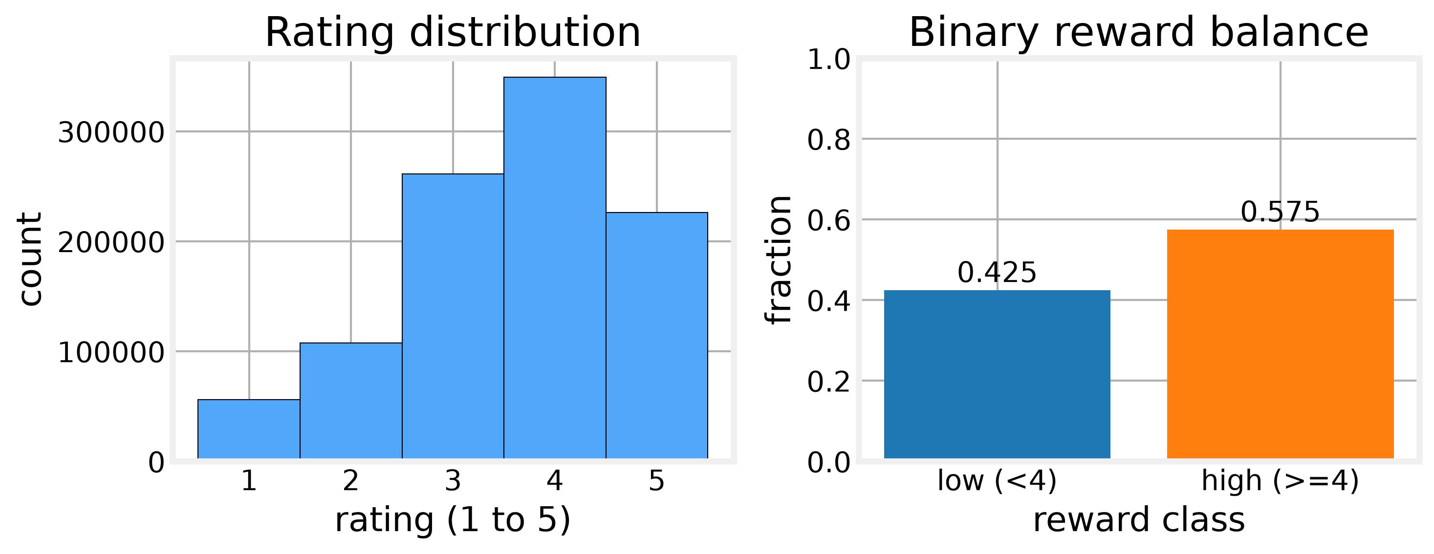
The left panel shows the familiar J-shape of movie ratings, piled up at 4 and 5. The right panel shows the consequence for us: the two reward classes sit at roughly 0.42 and 0.58, close enough to balanced that a hit rate is a fair score.
Two more findings shape the design. Age is stored as buckets, from under 18 up to 56 and over, and we use five of them as our contexts. The reward varies by age and by movie, so a policy that keeps separate estimates per age group has something to gain. We use per-movie arms because genre breadth does not identify a single movie.
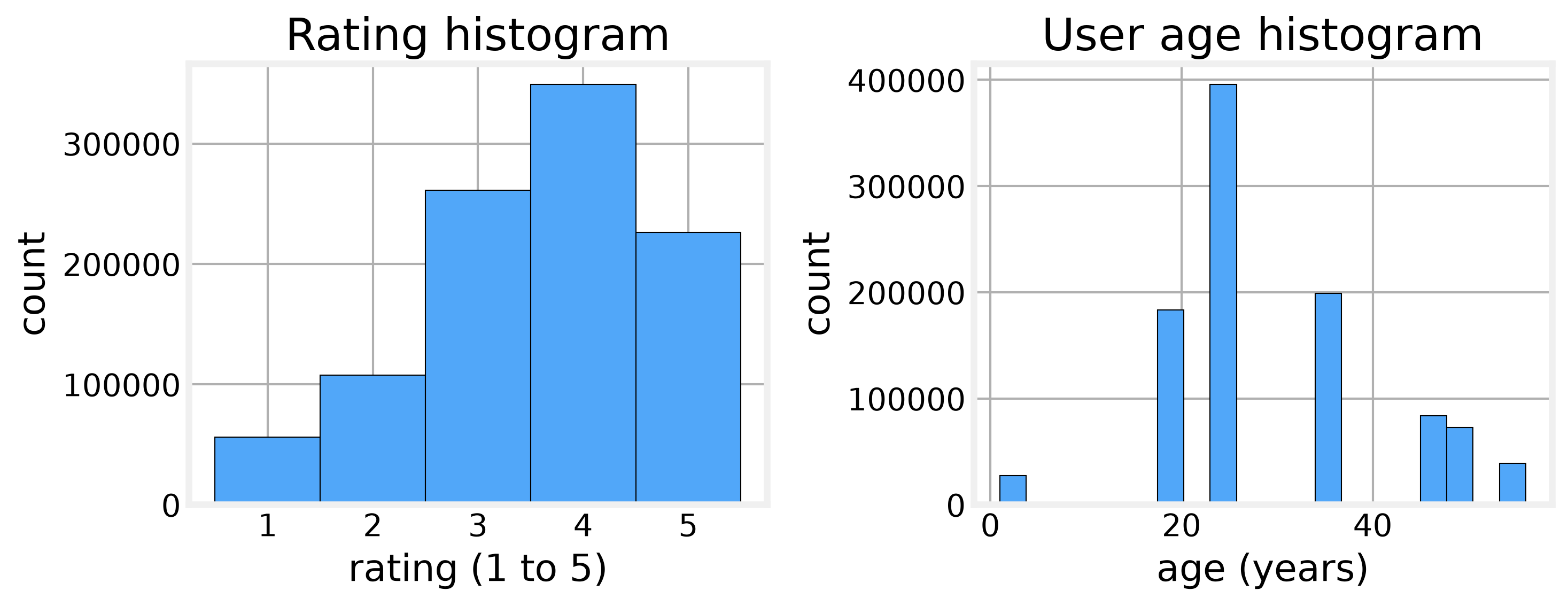
Users cluster in the 25 to 34 age bucket, so middle buckets carry most evidence and edge buckets need smoothing.
Setting up the replay
We cannot run a live experiment, so we replay one. We pick the 12 most-rated movies as our arms, so every arm has enough logged feedback to estimate from. We bucket users into five age contexts, split users 70/30 into train and test, and confirm the two sets share zero users. Test users only supply contexts, never reward estimates, so there is no leakage from the people we are evaluating on.
The ground truth is a smoothed reward table, one probability per context and arm, built from the training rows with Beta(1, 1) smoothing. That smoothing keeps unseen context-arm cells at 0.5 instead of zero, which matters because a few cells are sparse. The spread from 0.6 to 0.935 means arm choice changes expected reward by up to 0.335 in a context. The strongest arm by average probability is Raiders of the Lost Ark (1981).
With the table fixed, the simulation is simple. At each step we draw a context from the test users, ask the policy which arm to pull, flip a coin against the true probability for that context and arm, and hand the reward back. Regret at each step is the best probability available in that context minus the probability of the arm we chose. Summed over 12,000 steps, that gives the cumulative regret curve, and the lower the curve the better the policy spent its pulls.