Stochastic Blog

First classifiers and how to score them

In Post 10 we learned how to split data into training, validation, and test sets, and in Posts 3 and 4 we built our first regression models and baselines. Now we take the next step: training our first real classifiers on the UCI Adult Census Income dataset, where we predict whether someone earns more than 50K a year. By the end of this post we will have a pruned decision tree that reaches an area under the ROC curve (AUC) of 0.903 on the test set, and we will understand why accuracy alone would have misled us at every turn. The through-line of this post is the difference between ranking and deciding: classifiers can order people by income likelihood, but turning that order into a yes or no prediction requires a threshold, and every threshold tells a different story.

We build three families of classifiers on the Adult data, score them with metrics that expose different failure modes, and then calibrate their probabilities so the numbers we output mean what they claim. The dataset gives us about 48,842 rows and 14 columns, a clean binary problem with numeric and categorical features, missing values, and a class imbalance we cannot ignore.

The data

Before any model, we inspect the raw data. The base rate of high earners, those making over 50K, sits at 24 percent, which means a model that predicts everyone earns less would be right 76 percent of the time. That number becomes our floor: any classifier must beat it to earn its place. Missing values are confined to three categorical columns, workclass, occupation, and native_country, and we impute them with the mode in the pipeline. We drop fnlwgt, which is a sampling weight rather than a predictive feature, and we drop education because education_num carries the same information as a number.

The class imbalance is visible in Figure 1.

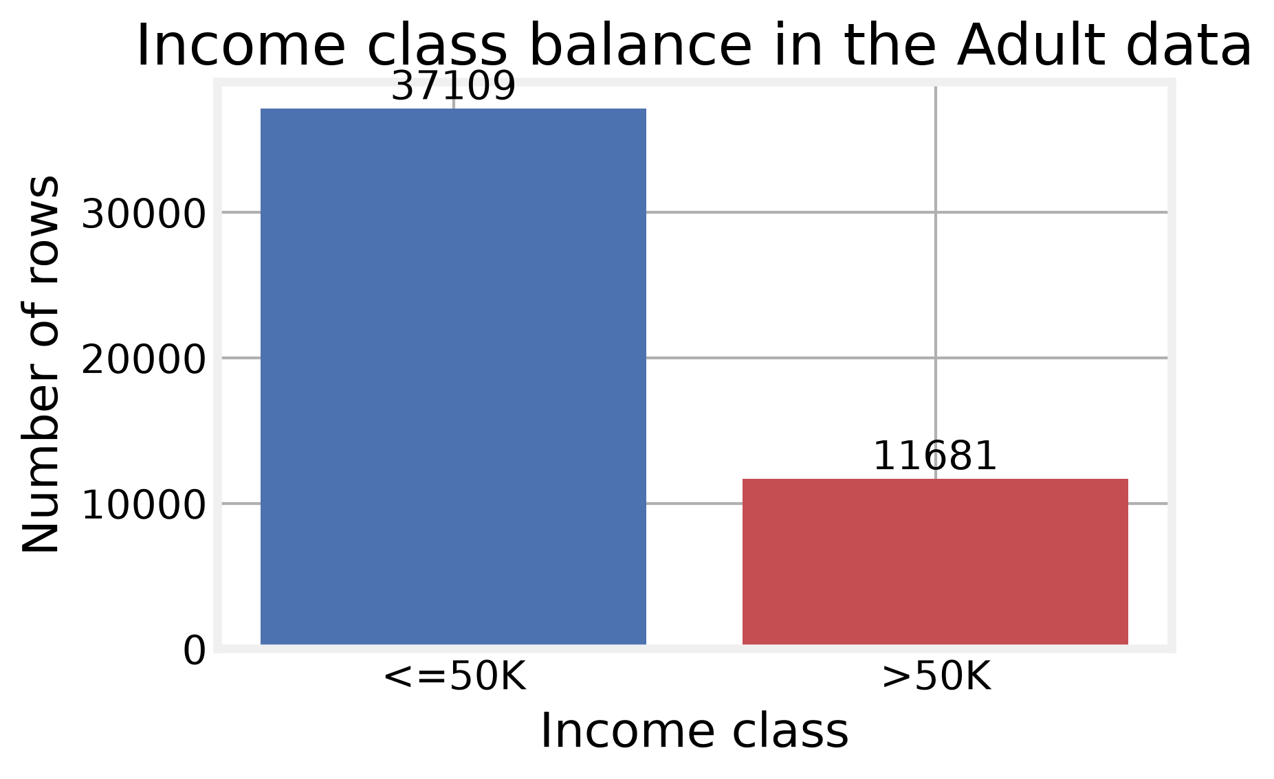
Figure 1: only 24% of rows are high earners, so a constant low-earner prediction would be right 76% of the time

The numeric features show the expected skews. capital_gain and capital_loss are zero-inflated, with most people having no capital activity at all, and hours_per_week has over 13,000 values beyond 1.5 times the interquartile range from the quartiles. We leave them unclipped; the tree-based and distance-based models we are about to train can handle the shape. The categorical columns have long tails, so we one-hot encode with handle_unknown='ignore', which is enough at this data size.

The histograms in Figure 2 make those skews concrete.

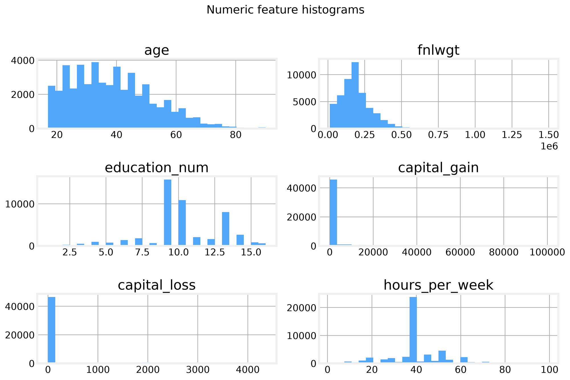
Figure 2: capital gain and loss are zero-inflated, and hours per week has a long right tail

The preprocessing pipeline combines a median imputer and standard scaler for the five numeric features, and a mode imputer with one-hot encoding for the seven categorical ones. After fitting on the training split, we end up with 88 encoded features, and we hold out 12,198 rows for the final test, 10,978 for validation, and 25,614 for training.

Starter models

With the encoding done, the first model we try is k-Nearest Neighbors, the lazy classifier: it stores the training rows and assigns a class by majority vote among the nearest neighbors. Distance metrics define what nearby means, so we try both Euclidean and Manhattan distance on a 10,000-row subset stratified to preserve the 76/24 class split, because a full 25,614 by 88 distance search is too slow for a laptop demo.

# kNN votes by majority among the k closest training rows
knn_euclidean = KNeighborsClassifier(n_neighbors=5, metric='euclidean').fit(X_knn_enc, y_knn)
knn_manhattan = KNeighborsClassifier(n_neighbors=5, metric='manhattan').fit(X_knn_enc, y_knn)

Both beat the baseline. Euclidean reaches 83.58 percent validation accuracy and Manhattan 83.38 percent, a small gap that tells us the geometry of the feature space is not particularly sensitive to the distance definition. The perceptron, our first linear classifier, does worse at 70.87 percent, below the 76 percent baseline; class_weight='balanced' keeps it from predicting the majority class for everyone, but that does not beat the constant predictor.

Polynomial regression serves as a reminder that linear models can be made flexible with polynomial features, but its raw scores are not probabilities. On validation, the degree-2 polynomial pipeline produces scores ranging from negative 0.443 to 1.881, and thresholding at 0.5 gives 81.75 percent accuracy. The sigmoid link function maps a real score to the interval between zero and one, which is why we will need it later for calibration.

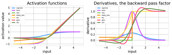
Figure 3 shows the shape of that mapping.

Figure 3: the sigmoid compresses any real score into a probability between 0 and 1

The perceptron is fast and linear, but it only returns decision scores, not probabilities. That limitation will matter when we compare models with probability-based metrics, and it sets up the calibration section at the end.

Decision trees

The perceptron showed that linear scores are not enough; a decision tree loosens that assumption by splitting rows with yes or no rules. The CART algorithm grows one binary split at a time by minimizing impurity. Gini impurity, the chance a random row in a node is mislabeled if labeled by that node's class proportions, is the default measure; information gain is the entropy-based alternative. We train a full tree first, and it grows to 8,975 nodes with a root Gini of 0.3642, which reflects the 24 percent base rate. The unpruned tree reaches 82.33 percent validation accuracy and has 8,975 nodes; that validation score is lower than the depth-4 tree's 84.9 percent, a sign of overfitting.

Depth-4 trees are easier to inspect. Gini and entropy give nearly identical results, 84.93 and 84.97 percent respectively, which tells us the choice of impurity measure matters little here. Cost-complexity pruning trims weak branches after the tree is grown, trading training fit for validation accuracy. We sweep the complexity parameter and find the best value at 0.000123, which produces a tree with only 235 nodes and 86.25 percent validation accuracy, the best tree result so far.

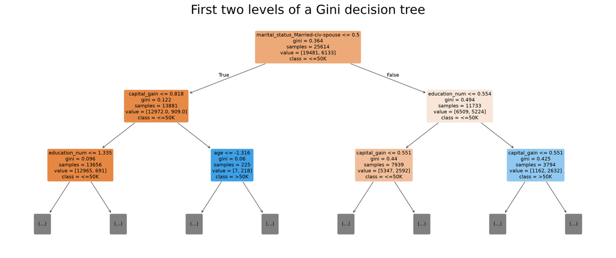
Figure 4 shows the first two levels of the Gini tree.

Figure 4: the first splits separate on capital gain and marital status, the two strongest signals

The pruned tree is the model we carry forward. It is small enough to inspect, accurate enough to beat the baseline by ten points, and its probability output will let us tune thresholds and calibrate.

Classification metrics

How good is the pruned tree? Start with the four counts in its confusion matrix, which counts true positives, false positives, true negatives, and false negatives. For the pruned tree at the default 0.5 threshold, we get 7,755 true negatives, 595 false positives, 914 false negatives, and 1,714 true positives. Precision is the share of positive predictions that are correct, 74.23 percent here. Recall is the share of real positives we found, 65.22 percent. The F1 score harmonizes the two at 0.6943.

Figure 5 visualizes those counts.

Figure 5: the pruned tree at threshold 0.5 misses more positives than it catches, which motivates threshold tuning

Matthews correlation coefficient summarizes the whole 2x2 table at 0.6083, and Cohen's kappa measures agreement above chance at 0.6062. These two agree closely, which is reassuring. But the default threshold is arbitrary, and threshold tuning changes the point at which a probability becomes a positive prediction. We sweep thresholds from 0.10 to 0.90 and find that the best F1 comes at 0.40, where it reaches 0.7072. Applying the 0.40 threshold to the test set gives an F1 of 0.700.

# Sweep the decision threshold to balance precision and recall
for t in thresholds:
    pred = (proba_tree >= t).astype(int)
    f1s.append(f1_score(y_val, pred, zero_division=0))

Lowering the threshold from 0.5 to 0.4 catches more true positives at the cost of more false positives, and the F1 gain of about one point is modest but real. The lesson is that the default threshold of 0.5 is just a convention, not a law.

Score curves

A threshold sweep only examines one operating point; ROC curves look at every threshold at once. ROC curves plot true positive rate against false positive rate over all thresholds, and AUC is the area under that curve. We compare the Euclidean kNN, the pruned tree, and the perceptron on the untouched test set. The tree and kNN both achieve AUC around 0.90, while the perceptron trails noticeably.

Figure 6 shows the ROC comparison.

Figure 6: the tree and kNN hug the top-left corner, while the perceptron's curve bows toward the diagonal

Precision-recall curves keep precision on the y-axis and recall on the x-axis, and average precision summarizes the curve. Here the gap between models grows because the positive class is rare. The perceptron's PR curve collapses toward the base rate, while the tree and kNN hold up better. Log loss and Brier score measure how close predicted probabilities are to observed outcomes, not just how well the model ranks rows. The pruned tree scores a log loss of 0.3703 and a Brier of 0.0976, while kNN scores 1.4233 and 0.1192. The kNN's log loss of 1.4233, far worse than the tree's 0.3703, reveals that its probability estimates are badly off.

Probability calibration

The raw tree is overconfident in some bins, meaning it predicts probabilities that are higher than the observed frequencies. Platt scaling fits a sigmoid to the raw scores so they become probabilities, and isotonic calibration fits a non-decreasing step function instead. We calibrate on validation data so the test set remains untouched.

# Calibrate on validation so the test set stays untouched
platt_cal = CalibratedClassifierCV(pruned_tree, method='sigmoid', cv=2)
iso_cal = CalibratedClassifierCV(pruned_tree, method='isotonic', cv=2)

The results surprise us. Starting from those same baselines, Platt scaling makes both worse: 0.1246 and 0.4044; isotonic also degrades them, to 0.1225 and 0.3963.

Figure 7 shows the calibration curves.

Figure 7: the raw tree already sits close to the diagonal, and calibration pushes it away

The calibration curves show the raw tree is already reasonably close to the diagonal, and the calibration methods overcorrect. This is an honest negative result: calibration is not always an improvement. The raw tree's probability estimates are good enough that forcing them through another transformation adds noise rather than removing bias.

Closing

We started with a 24 percent base rate and ended with a pruned tree that reaches an AUC of 0.903 and an F1 of 0.700 at a threshold of 0.40 on the test set. The EDA findings drove every decision: the imbalance pushed us toward precision and recall, the missing values shaped the imputation strategy, and the zero-inflated capital features stayed unclipped because the tree handles them. The through-line holds: ranking the data was easy, but deciding where to cut required threshold tuning, and calibrating the probabilities turned out to be unnecessary for this model.

The notebook simplifies a few things. We train kNN on a 10,000-row subset rather than the full training set, we use a single validation split instead of cross-validation, and we do not tune hyperparameters beyond the pruning sweep. A production version would use cross-validated threshold selection and would check whether the calibration degradation persists across different random seeds.

The question this post leaves open is whether a single tree is the best we can do. The pruned tree has 235 nodes, and its depth-4 cousin is easy to read, but both are limited by the greedy nature of CART. The next post answers that question directly: we move from trees to forests with bagging and random forests, where many weak trees combine into a stronger predictor.

Exercises. Change the kNN distance metric to Minkowski with p=3 and compare it to Euclidean and Manhattan. Add min_samples_leaf=50 to the decision tree and compare its cost-complexity pruning path to the default tree. Use the validation threshold sweep to pick a threshold that gives at least 70 percent precision, then evaluate recall and F1 at that threshold on the test set. Implement Platt scaling by hand with LogisticRegression on the tree decision scores, and compare the result to CalibratedClassifierCV with method='sigmoid'. Use cross_val_predict on the training set to generate out-of-fold probabilities for isotonic calibration, then check whether calibration still improves the test Brier score.