Bayesian modeling with MCMC

In Post 3 we fit a least-squares line to a dataset and read a single number off it. In Post 4 we learned to distrust that number until we saw it on held-out rows. This post builds the machinery that replaces the single number with a distribution. We will write a prior, a likelihood, and a posterior, update one into the other in closed form, then sample a posterior we cannot integrate with six different algorithms and score every one of them against the exact answer. The through-line is a single question: how close does each sampler get to the truth we already know? On California housing prices, the conjugate posterior mean for the intercept is 1.9505 and the best sampler lands within 0.00043 of it. The worst one is not far behind, and the reason why is the whole lesson.

The data and what it hides

We work with California Housing, served by scikit-learn through fetch_california_housing. It is 20,640 rows, eight numeric features, one numeric target, about 1.5 MB in memory, and no categorical column anywhere. The target is MedHouseVal, median house value in units of 100,000 USD. The features mix income, room counts, age, population, and location, which is exactly the kind of table where coefficients come out at wildly different scales and a shared prior has to be chosen with care.

Before any model, we look. Five raw rows come first, because transforms hide faults. There are no missing values in any of the nine columns, so nothing is imputed and no row is dropped for gaps. There are zero duplicate rows. The one thing that does need a decision is the target ceiling: MedHouseVal is capped at 5.00001, and 965 rows, 4.7 percent of the table, sit exactly at that cap. That is a recording artifact, not a real price. A cap flattens the top of the price range and would bias every coefficient downward, so we drop those rows and keep the rest.

Figure 1 plots histograms of all nine fields, clipped at the 0.5 and 99.5 percentiles.

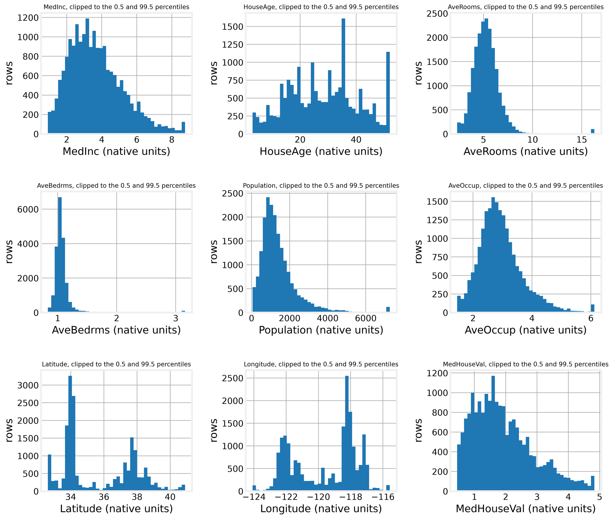
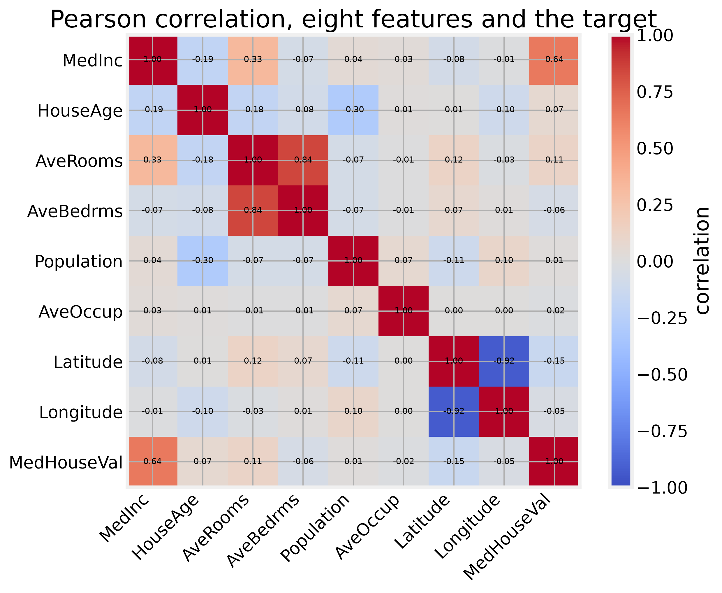
The distributions tell us what the model needs. MedInc is the strongest linear correlate of price, and Latitude and Longitude follow close behind, so the model needs income and location together. AveRooms, Population, and AveOccup are heavy tailed, a few extreme rows stretch each distribution, which means a regression on raw counts would be dominated by a handful of rows. The outlier shares differ by orders of magnitude across fields, from zero percent for HouseAge to 6.9 percent for AveBedrms, which is another reason to standardize, rescale each feature to mean zero and standard deviation one, before putting a shared prior on the coefficients.

Figure 2 plots Pearson correlations, a measure of linear association that runs from -1 to 1.

The constant-mean baseline RMSE, root mean squared error, the average prediction error in target units, on the full table is 0.981, and that is the number every model below has to beat on held-out rows. For the sampling models we draw 5,000 rows with seed 42, because four Hamiltonian Monte Carlo chains (NUTS) on 19,000 rows would blow the CPU budget and 5,000 still resolves every coefficient. Train and test indices are disjoint by construction, asserted before fitting in the Monte Carlo sampling section.

Priors, likelihoods, posteriors

Bayes turns a guess into a distribution. A prior is a distribution over coefficients before seeing data. A likelihood is the probability of the data given coefficients. A posterior is the updated distribution after data. We write a prior over the unknown coefficients, write the likelihood of the data given those coefficients, then combine them into a posterior. The posterior is proportional to the likelihood times the prior. When the prior and the likelihood form a conjugate pair, the posterior has a closed form, and that is what Conjugate priors buy you. It also gives us an exact answer to check every sampler against.

The simplest case is one parameter: the mean price, with the spread of price treated as known. A normal prior, bell-shaped, plus a normal likelihood with known sigma, the standard deviation, gives a normal posterior, and the update is a short closed-form update. Precision here means one over the variance.

def mean_model_posterior(obs, prior_mu, prior_sd, sigma):
    """Normal prior plus normal likelihood with known sigma gives a normal posterior."""
    prior_prec = 1.0 / prior_sd ** 2
    like_prec = len(obs) / sigma ** 2
    post_prec = prior_prec + like_prec
    post_mu = (prior_prec * prior_mu + like_prec * obs.mean()) / post_prec
    return post_mu, post_prec ** -0.5

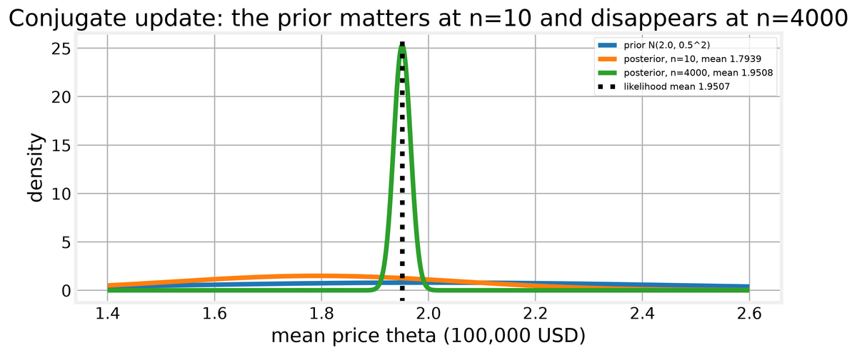
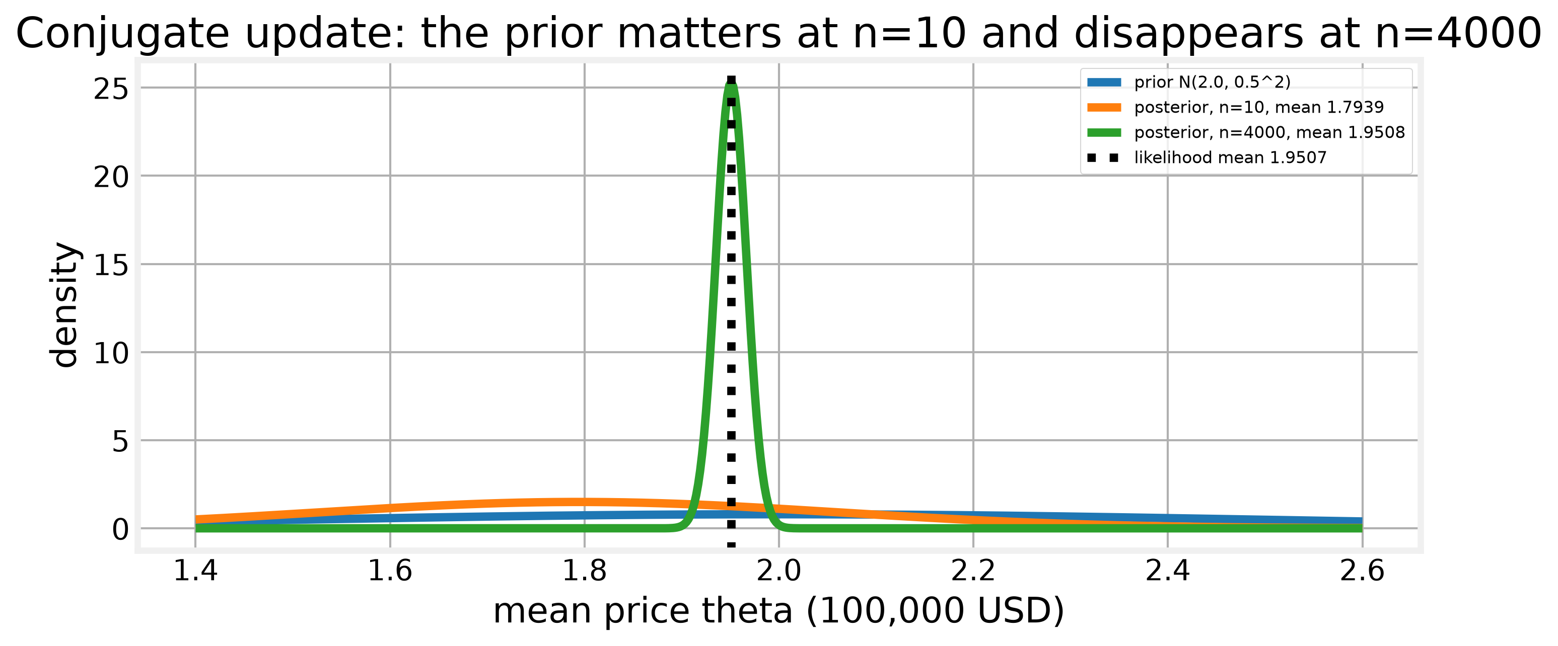
We set the prior at 2.0 with sd 0.5, a loose guess that the price level sits near 200,000 USD. At n=10 the likelihood is wide, so the posterior lands between the prior and the data and the prior visibly pulls the mean. At n=4000 the likelihood precision dominates by roughly a factor of 400, the posterior mean matches the sample mean to the third decimal, and the posterior sd collapses to 0.01576. The gap between the posterior mean and the likelihood mean is 0.00005. With plenty of data a weakly informative prior is nearly irrelevant, which is exactly why it is safe to state one.

Bayes factors compare two models by their approximate marginal likelihoods, the probability of the data under a model. Using the BIC shortcut, an approximate fit score that penalizes parameters, the intercept-only model scores a BIC of -14.8, the MedInc-only model scores -2145.53, and the five-feature model scores -3234.40. The log10 Bayes factor against the intercept-only model is 462.69 for MedInc alone and 699.13 for the full model, both far above the threshold of 2 that counts as decisive on the Jeffreys scale, a convention for reading Bayes-factor strength. The five-feature model fits better and pays a six-parameter penalty. Because Bayes factors scale with n, these Bayes factors say nothing about how much better the model predicts on new houses. The held-out RMSE at the end of the notebook is the honest comparison.