Hidden states, filters, and Gaussian Processes

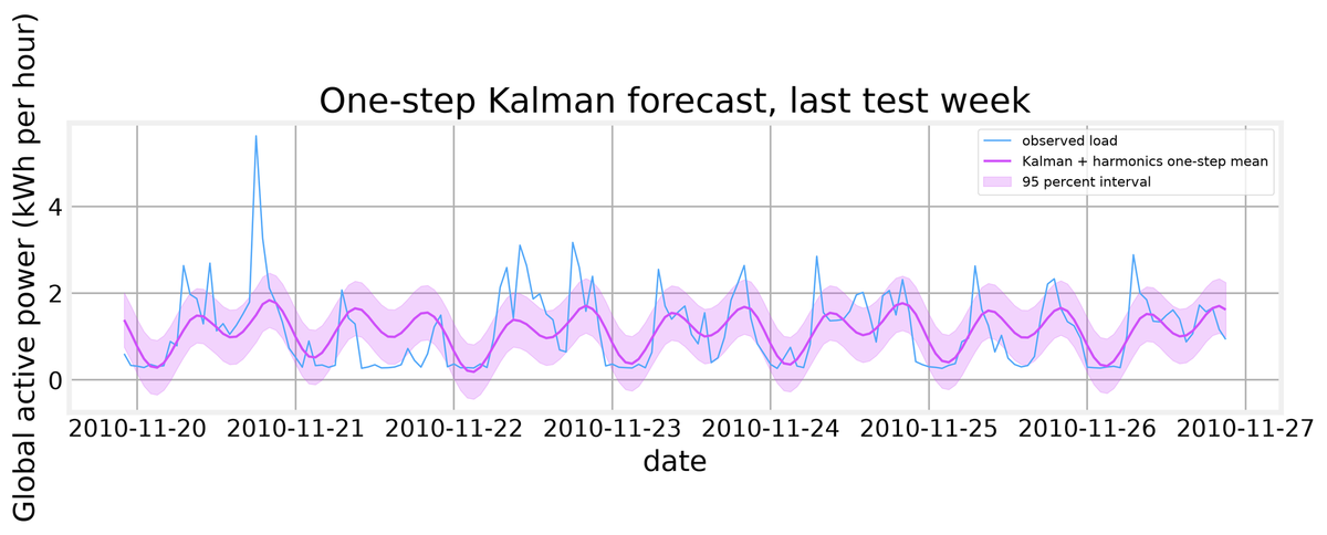
Post 20 gave us the probability toolkit, and Post 21 pushed uncertainty into deep models. This post keeps the same question, uncertainty, and moves it onto sequences and functions. We will read a temporal model as a graph, fit a Gaussian hidden Markov model to hourly power use, run four different filters on one nonlinear problem, fit a Gaussian Process to daily load, cluster daily shapes with a Dirichlet process, and quantify forecast uncertainty four ways. The concrete result we reach: a three-state chain decodes the high-load regime at 0.905 balanced accuracy, and a Kalman filter with daily harmonics cuts the level-plus-trend filter's error from 0.7813 to 0.6657 kWh per hour, though persistence remains slightly better at 0.6618. The through-line is the same idea in every section. A hidden state is a small set of numbers we never observe, and every method here is a different way of guessing those numbers from what we can see.

We work with the UCI Household Electric Power Consumption dataset, about 2 million one-minute readings from a single home between December 2006 and November 2010. It is long, strongly seasonal, and non-stationary, which is exactly what makes hidden states worth fitting and what makes a Gaussian Process a fair test. The notebook runs end to end on a CUDA device, with numpy 2.5.1, pandas 2.3.3, scikit-learn 1.9.0, statsmodels 0.14.6, torch 2.13.0, and pymc 6.3.2.

Reading the data

Before any model, we look. The file parses to 2,075,259 rows on a one-minute grid with seven float measurements, and it loads in 2.9 seconds. Two columns are traps. Global_intensity is defined as Global_active_power times 1000 divided by Voltage, and the median absolute gap between the implied and recorded values is 0.0805, with 98.23 percent of minutes within one amp. Together, Global_intensity and Voltage algebraically reconstruct the target, so both are leakage and stay out of every model frame below. Missing target values affect 1.252 percent of minutes, and the hourly mean skips them, leaving only 421 empty hours out of 34,168. No imputation is needed anywhere.

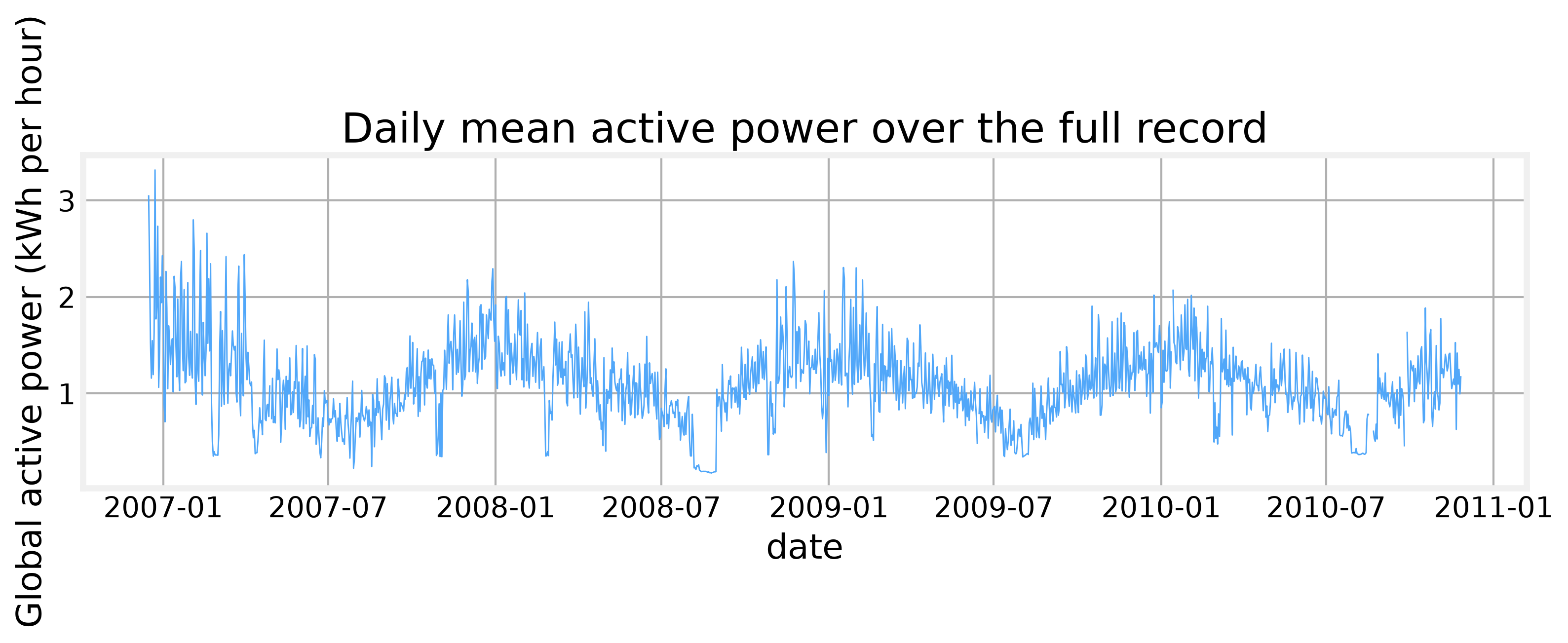
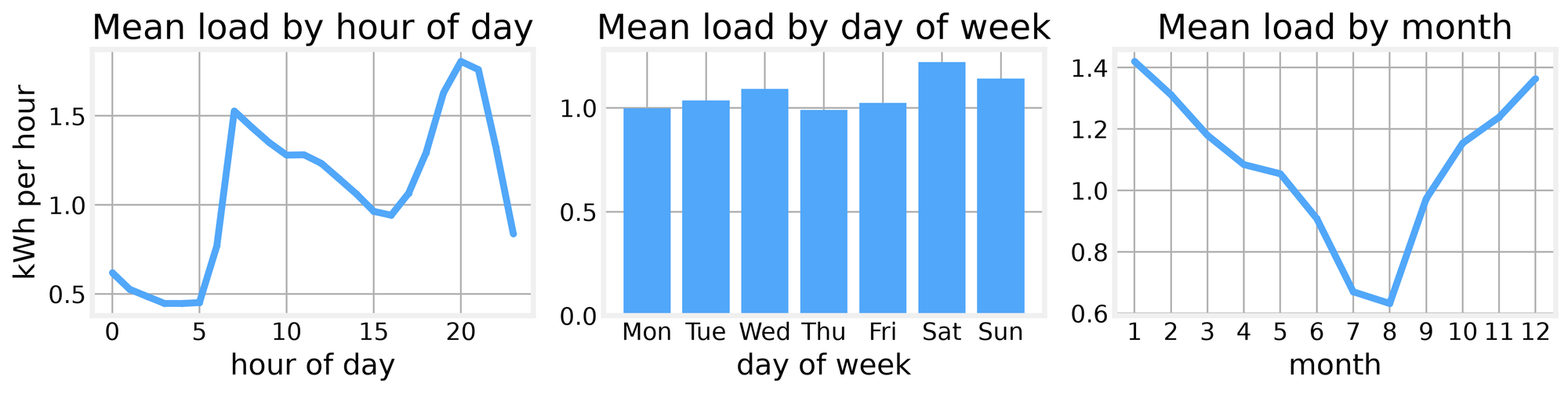
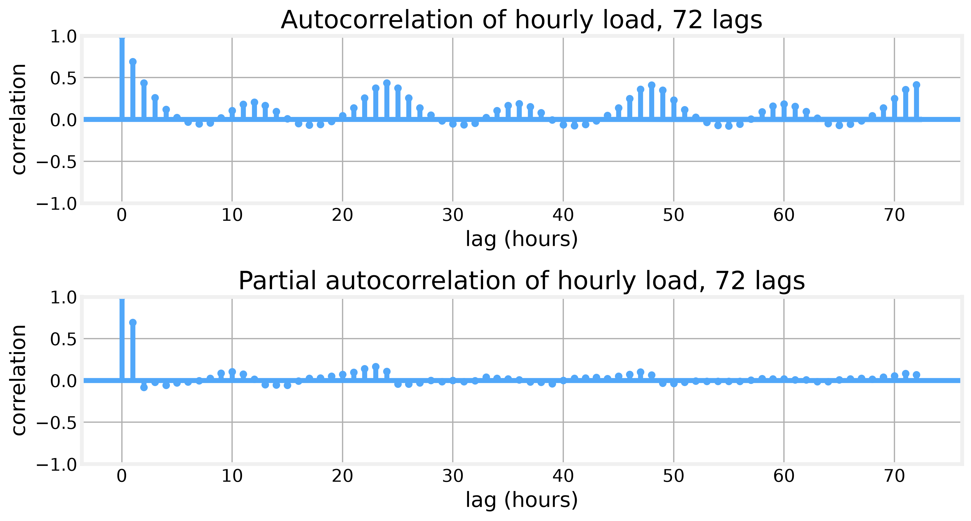
The daily cycle dominates everything else. The peak hour is 20 with a mean of 1.806 kWh per hour, the trough is hour 4 at 0.446, and the peak-to-trough ratio is 4.05. The level moves by a factor of four inside every day, which is precisely the structure a hidden state can capture. The weekly cycle is much weaker, with a weekend-minus-weekday gap of 0.153 kWh per hour, and seasonality is large, with winter sitting 0.629 kWh per hour above summer. The autocorrelation at lags 1, 24, and 48 hours is 0.692, 0.438, and 0.410, and the partial autocorrelation spikes at lag 24. Autocorrelation is correlation with a lagged copy of the series. Partial autocorrelation removes the shorter lags first. A random walk plus daily harmonics is a sensible state space model, and that is what we build.

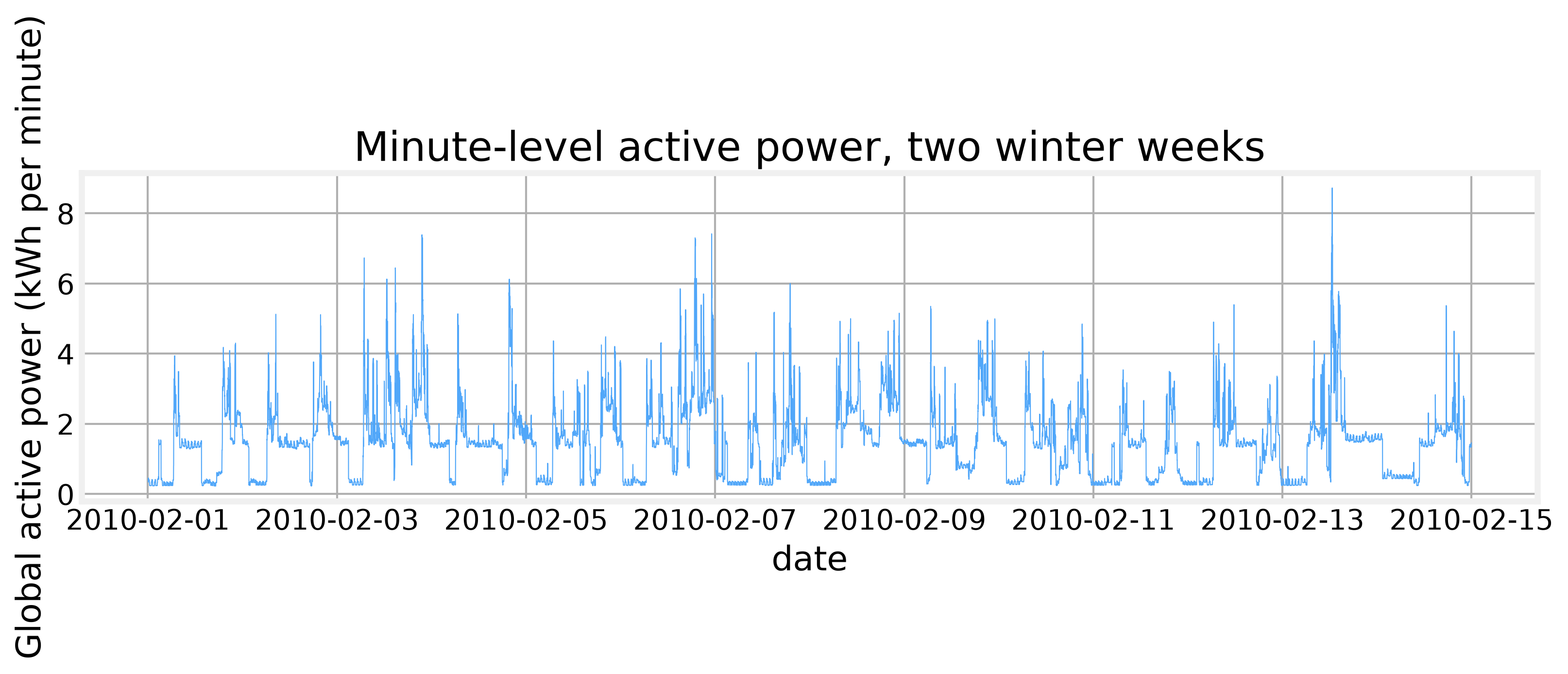
The six figures below establish the shape of the problem before any model touches it: the threshold that defines the high-load label, the seasonal swing across the full record, the three calendar cycles side by side, the fine structure the hourly mean hides, the lag structure that motivates daily harmonics, and the split we hold fixed for everything that follows.

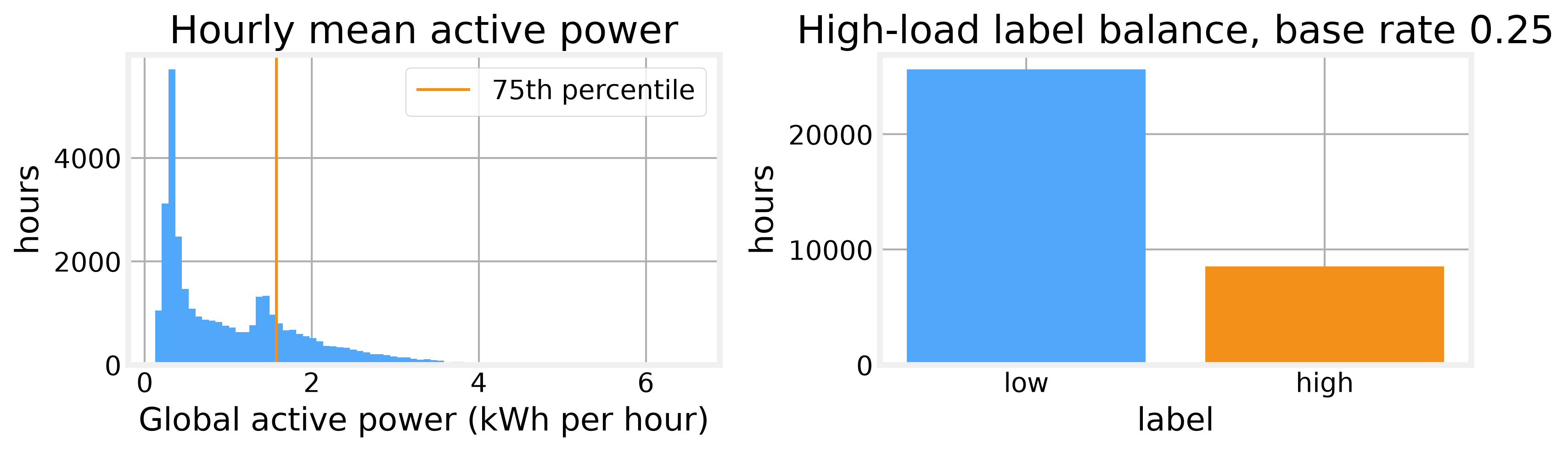
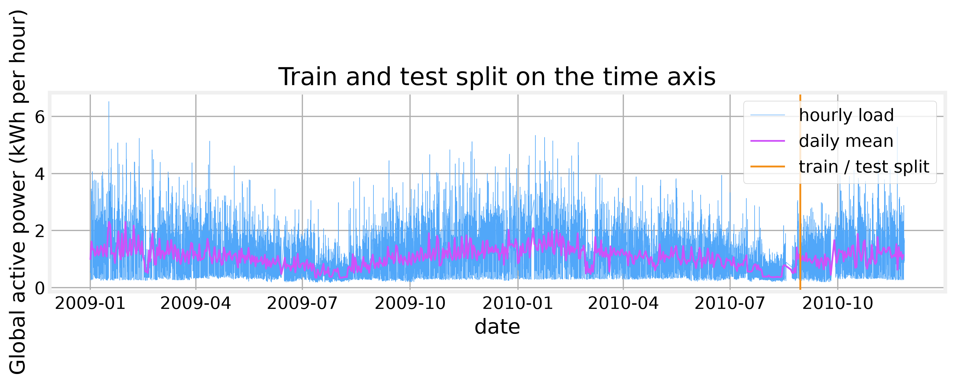
We split at 2010-08-30, giving 14,272 training hours and 2,047 test hours, plus 600 training days and 87 test days. The high-load threshold is computed on the training window only, at 1.535 kWh per hour, so the label carries no future information. Every model below uses this same split.

Graphical models

With the split fixed and the daily cycle established, the next question is how to represent dependence among variables. A Bayesian network factors a joint distribution over a directed acyclic graph, and in a sequence that chain structure is exactly what makes exact inference cheap. d-separation is the graph rule for reading conditional independence off the picture. A path through a chain or a fork is blocked once we condition on the middle node, but a path through a collider is blocked until we condition on the collider. That asymmetry explains why conditioning can create dependence as well as remove it. A Markov random field drops the direction and keeps a product of non-negative potentials over cliques, and belief propagation sends messages along the edges, converging in one forward and one backward sweep on a tree.

We can test the collider rule directly on the training hours. Weekend and evening peak hour are independent on their own, and the marginal mutual information is essentially zero at the sixth decimal. Once we condition on the high-load collider, the same pair becomes dependent, and the conditional mutual information is 0.00026. d-separation predicted that, and the data confirms it.