Augmentation, transfer, and smaller models

In Post 23 we closed the gap between a model that memorizes and a model that generalizes, using weight decay, dropout, and early stopping to hold the bias-variance balance. That gave us a network that fits CIFAR-10 without falling apart on the test set. But a well-regularized model is still a model trained from scratch, on one task, at full size. This post asks a different question: what can we do with a network besides train it once and hope? We will bend the training data, reuse a network trained on one task to help another, keep a model from forgetting what it knew, and shrink the whole thing down. The concrete payoff comes early: a linear probe (a linear classifier trained on frozen features) from a five-class source model (a network trained only on the first five classes) reaches 0.470 on the full ten-class test set, against 0.407 for the same probe on random features. That 0.062 gap is knowledge we did not have to retrain for.

Think of the whole post as a single workshop with one small CNN on the bench. We build it once, then we ask how many different ways we can get more out of it: more from the same images, more from a previous training run, more from a teacher (a trained model that supplies soft labels), and more from fewer weights. The dataset is CIFAR-10, pulled with torchvision into a local cache, and we work on a subsample so every experiment fits a laptop budget.

The data on the bench

CIFAR-10 is 60,000 color images of 32x32 pixels, split 50,000 train and 10,000 test across ten balanced classes. The raw arrays cost about 184.8 MB in memory and the download is about 170.5 MB on disk. Ten balanced classes means the base rate is 0.10, so any accuracy above that is signal. We subsample to 6,000 train and 2,000 test images with seed 42, which gives roughly a tenfold speed-up while keeping the class balance intact.

Before any modeling, we look at the pixels. The first thing to check is whether the images are what the labels claim.

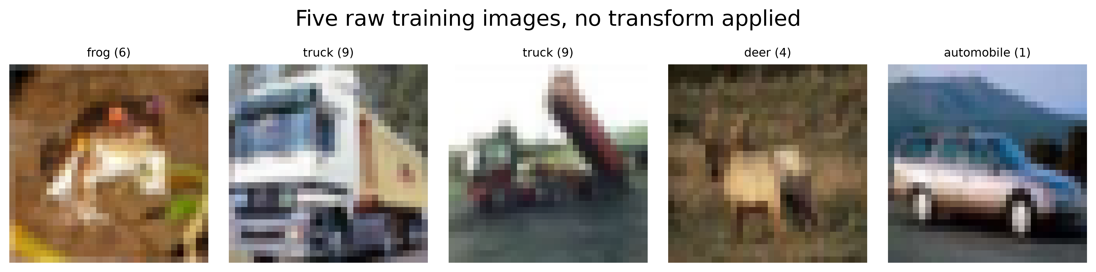
The five raw images come out as frog, truck, truck, deer, and automobile, each 32x32x3 in uint8. No transform is hiding a resizing fault or a mislabeled row. The class counts are perfectly even at 1,000 per class on the test split, so the majority-class base rate is exactly 0.100.

We also scan for duplicates, hashing every image with md5, a checksum that turns each image's pixel bytes into a short fingerprint. There are zero exact duplicates inside train, zero inside test, and zero test images that also appear in train. That last number matters: if a test image had leaked into the training set, our reported accuracy would be inflated by memorized rows. It is not.

The channel statistics come from the data, not from a quoted constant. The per-channel mean is [0.4913, 0.4814, 0.4445] and the per-channel std is [0.2476, 0.2445, 0.2627], computed over the first 5,000 training images. We will normalize with these exact values.

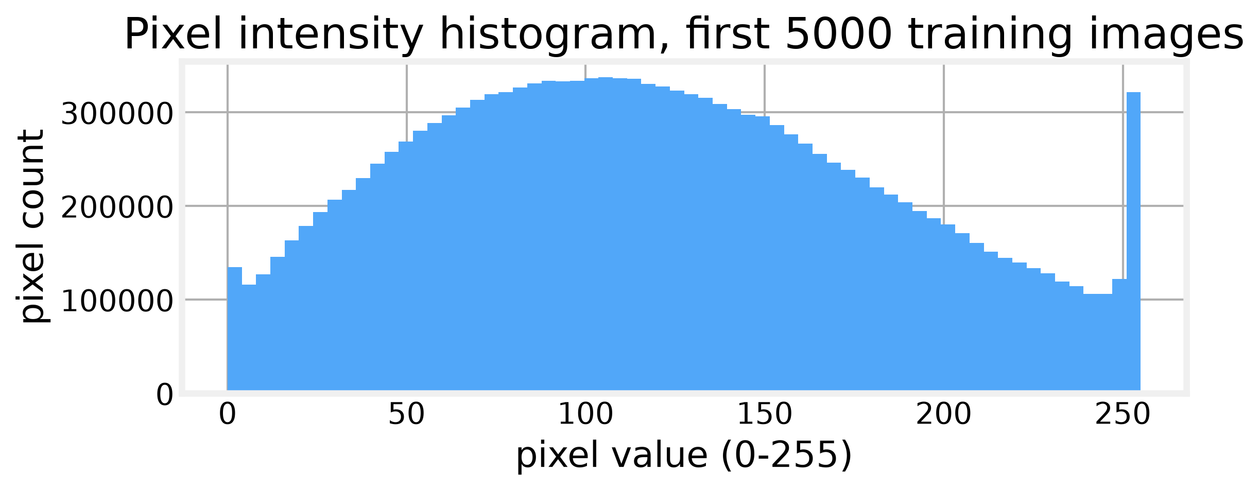
The intensity histogram is broad and roughly unimodal, spanning the full 0 to 255 range. There is no clipping at either end, so the images carry real variation rather than saturated blobs.

Two more findings shape everything downstream. First, the per-class grid shows a wide spread of pose, scale, and background inside every class, which is why augmentation has room to help. Second, the classes are visually close: cat and dog, deer and horse. That closeness is where soft targets and distillation will have meaningful information to transfer.

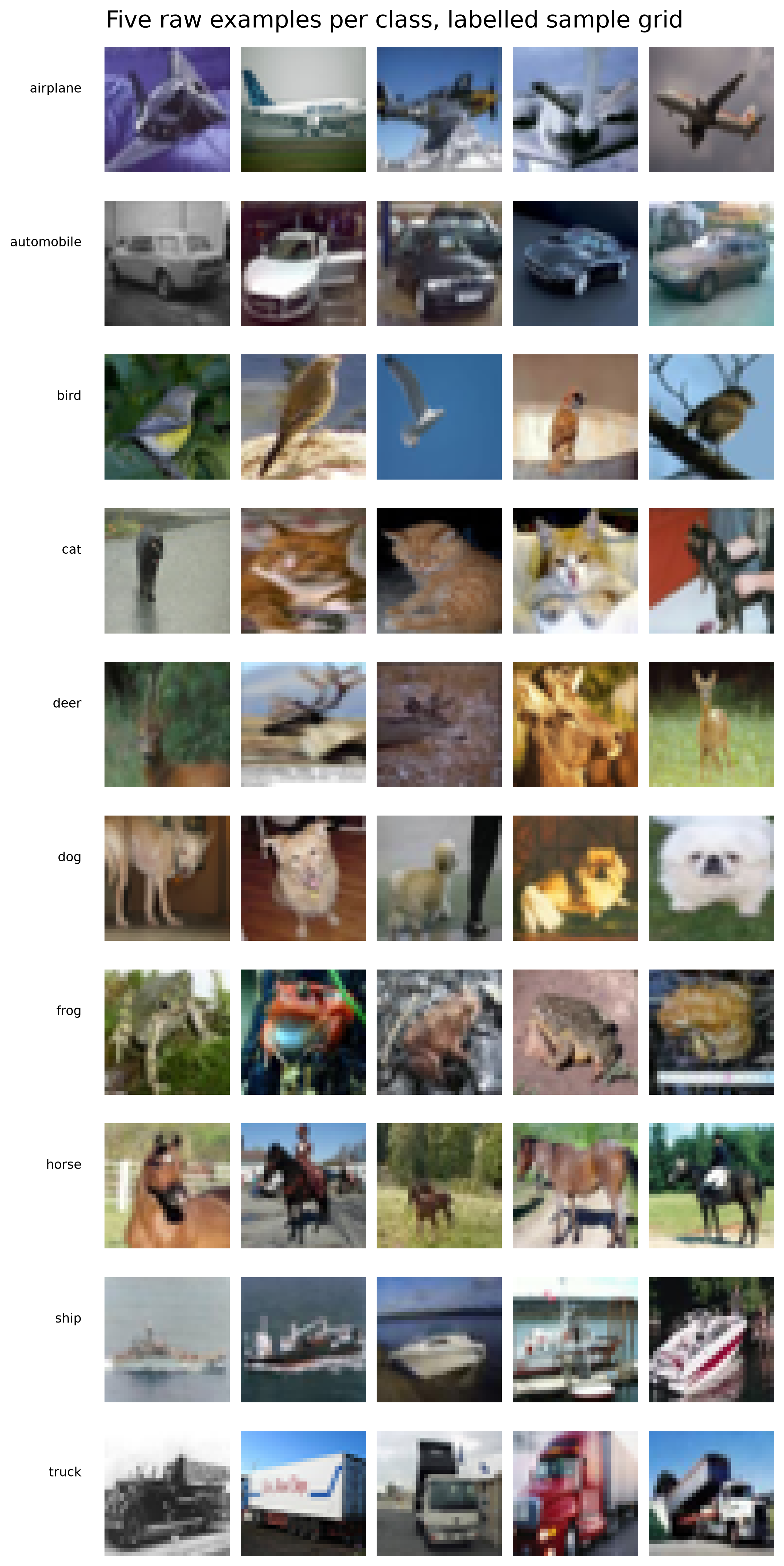
The grid makes the within-class spread obvious. Every class contains images at different scales, angles, and lighting, and a few rows are genuinely hard to read even for a human.

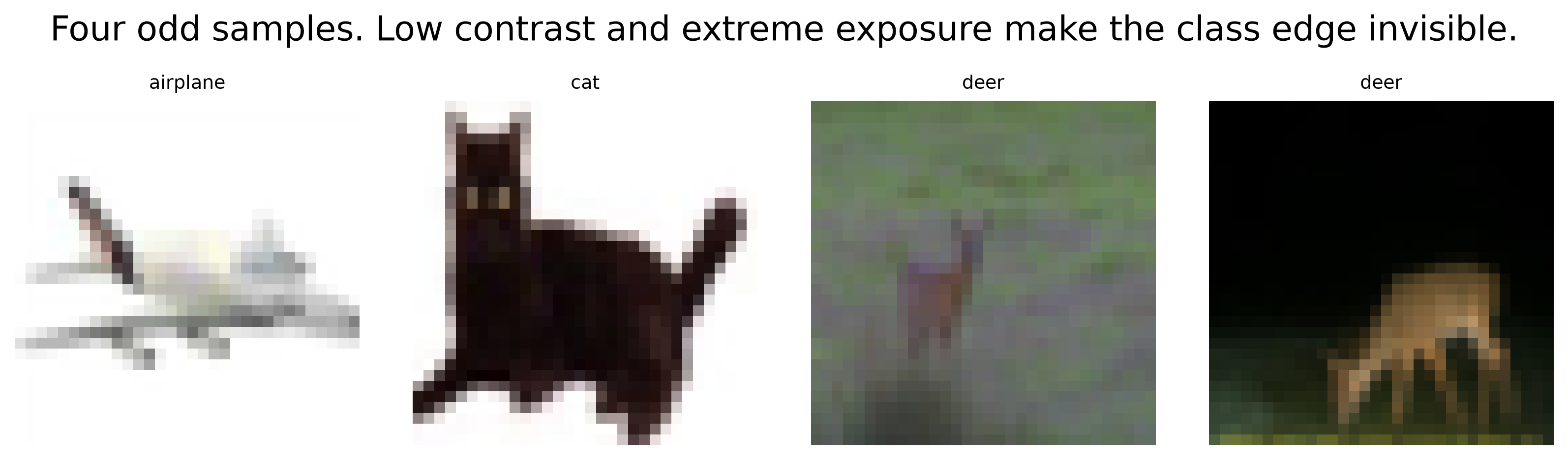
The odd samples confirm a floor on accuracy. Brightness percentiles run 48.8 at the 1st, 119.4 at the median, and 202.0 at the 99th. Contrast runs 25.2, 53.7, and 89.2. The washed-out and near-uniform patches carry almost no class information, so no model will get them all right.

Augmentation and curricula

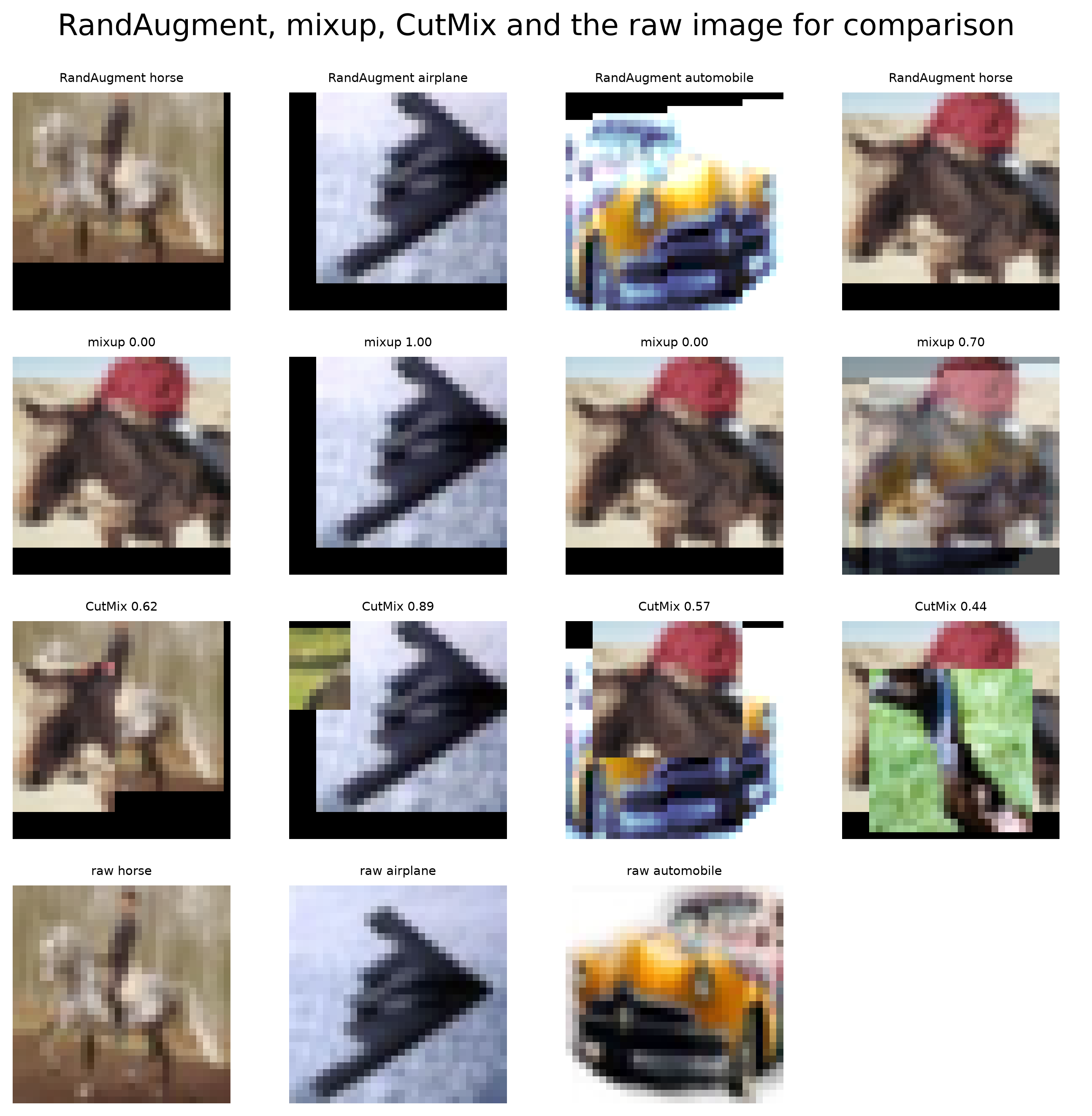
Because some images are unreadable and classes vary widely, the first lever is to change what the model sees. Augmentation changes the training distribution without changing the labels, and three image-space methods do most of the work. Mixup builds a convex combination (a weighted average whose weights are nonnegative and sum to one) of two images and trains on the same combination of one-hot labels (a vector with 1 on the true class and 0 elsewhere). CutMix pastes a rectangle from one image into another and scales the loss by the area. RandAugment applies a fixed number of random operations at a fixed magnitude, so the search space is two integers instead of thirty policies. Curriculum learning takes a different route: it reorders the training set, easy examples first, on the theory that early gradients should be clean.

The mixup and CutMix helpers are short enough to read directly. The idea in both is to blend two examples and blend their losses by the same weight.

def mixup_batch(x, y, alpha):
    lam = float(rng.beta(alpha, alpha))
    perm = torch.randperm(x.size(0), device=x.device)
    # Blend the images and keep both label sets, weighted by lam.
    return lam * x + (1.0 - lam) * x[perm], y, y[perm], lam

CutMix does the same thing but pastes a rectangle instead of blending pixels, then recomputes lam from the pasted area. Before spending any training time, we render the three augmentations side by side.