From bag-of-words to word vectors

In posts 23 and 24 we taught the machine to read: we loaded raw text, cleaned it with regular expressions, and ended up with a tidy table of documents. What we never did was decide what a document is once the cleaning is done. A string of characters is not something a model can multiply. This post builds the bridge from text to numbers, and it does so in three stages, each adding one mechanism the previous stage lacks. We start with the crudest representation, a bag of words, and we end with dense vectors where king sits a short step away from queen. The through-line is a single question that every method here answers a little better than the last: how much of a word's meaning can we recover from the company it keeps? The bag-of-words model says none of it, the n-gram model says a little, and the embeddings say enough that arithmetic on words starts to work.
We work on WikiText-2, the raw Wikipedia corpus, about 2 million tokens spread over roughly 36 thousand documents. A token is one running word instance. A type is one unique word form. It is small enough to train several embedding models on a laptop and large enough that the vocabulary, the frequency curve, and the n-gram counts behave like real text. Everything below runs on a single GPU, and every number comes straight from the notebook.
The corpus, and what exploratory data analysis (EDA) told us
Before any transform we look at the raw documents, because a transform hides empty lines, duplicated boilerplate, and truncation. The load gives us 21,580 rows across three columns, split, doc_id, and text, using 18.8 MB in memory. No text field is missing, so nothing is dropped for that reason. The split assignment is the only label this corpus carries, so that is the balance we plot.
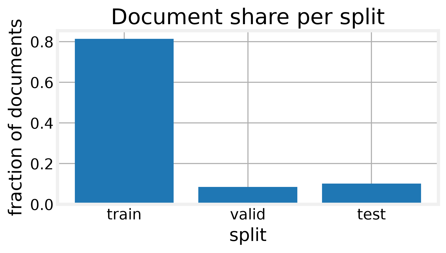
Train holds 81.35 percent of the documents, valid 8.53 percent, and test 10.12 percent. That imbalance is the base rate any classifier on this label would have to beat, and it is also a reminder that valid and test stay untouched while we train.
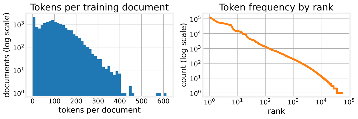
Two more findings shape everything downstream. First, duplicate documents exist inside each split, and there are 9 exact train/test overlaps. We drop 106 duplicates within their own split and remove the 9 leaking test rows, leaving 21,465 rows and a clean zero overlap between train and test. Second, the token frequency curve is close to a straight line on log-log axes, which means the type distribution is Zipfian: a few thousand types cover most tokens, and thousands of types occur exactly once.
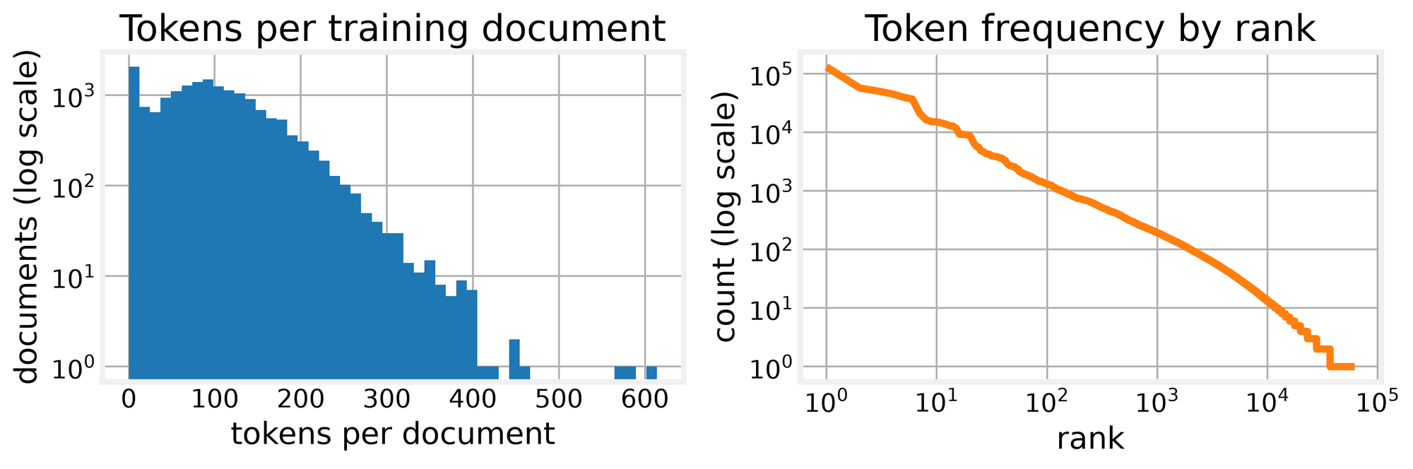
That long tail matters. After tokenizing the training split we have 1,680,658 tokens, 61,822 unique types, and only 36,909 types that occur at least twice. Embedding rows for the singletons would never receive enough gradient to move, so our embeddings use a count floor of 5. The Zipf curve is also why the out-of-vocabulary rate is worth measuring: against the full training vocabulary the test OOV rate is 0.0417, and against the count-2 vocabulary it rises to 0.0539. That number is the ceiling for any word-level model, and it is the reason subword units earn a place later in the post.
Text fundamentals
The OOV ceiling starts with the representation itself. A first representation treats a document as a bag of its words. Order disappears and only the counts survive. We can see the blindness directly: two sentences that share the same words in opposite order, the dog bit the man and the man bit the dog, produce a cosine similarity of 1.0, and cosine similarity measures the angle between two count vectors, so 1.0 means identical direction. Every later model in this notebook inherits that blindness unless it adds context back.
Weighting each count by how rare the word is across the corpus gives TF-IDF, where the weight is the term frequency times the IDF, the log of the total document count divided by the number of documents containing the term. On a 600-document sample of the real corpus, with min_df=2 (ignore terms that appear in fewer than two documents) to strip one-off boilerplate, we get a sparse matrix of 600 by 4,332 with 32,312 non-zero entries, and IDF values ranging from 1.14 to 6.3. The top terms per document are readable, which is why TF-IDF stays the default baseline for search and tagging.