Stochastic Blog

Linear models from least squares to quantiles

In the last few posts we built up the machinery of supervised learning from first principles, from nearest neighbors through decision trees and ensemble methods. Now we turn to the oldest and most enduring family in the toolbox: linear models. By the end of this post we will have fitted the major linear regression families to the California Housing dataset, watched our test error fall from a naive baseline of 1.1449 to a polynomial ridge model at 0.6877, and learned why the choice of loss function matters as much as the choice of model.

The through-line for this post is a simple one: every linear model is the same machine, and the only thing that changes is what we tell it to care about. Least squares cares about every error equally. Huber loss cares less about the outliers. Quantile regression cares about a specific slice of the distribution. The architecture stays fixed; the objective moves.

We work with the California Housing dataset throughout, 20,640 rows and 8 predictive features with MedHouseVal as our target in units of $100,000. It is a continuous regression problem with a heavy right tail and a hard cap near 5.0, which makes it ideal for exposing the differences between loss functions.

The data

Before any modeling, we inspect the raw data. The exploratory data analysis (EDA) reveals four findings that will shape everything that follows. First, MedHouseVal has a long right tail with 1,071 outliers by the 1.5 IQR rule, and the distribution is capped near 5.0. Second, MedInc has the strongest linear correlation with the target, which we will see dominate the coefficients in every model. Third, there are no missing values, so no imputation is needed. Fourth, AveOccup, Population, and AveRooms contain extreme outliers, which means scaling before any L1 or L2 penalized model is mandatory.

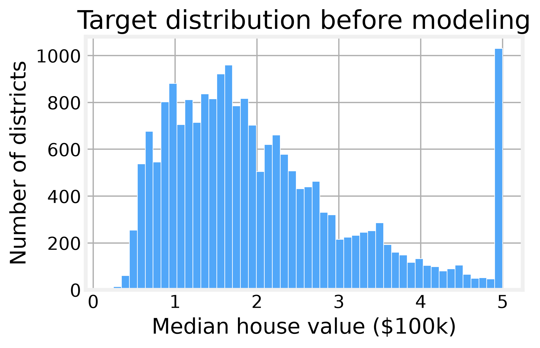
Figure 1 shows the target distribution.

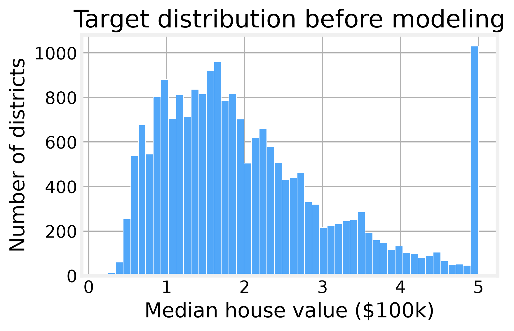
The target distribution shows a long right tail and a hard cap near 5.0, which will pull squared loss toward the top-coded districts

The histogram makes the story concrete. The mass of districts sits between 1 and 3, but a long tail stretches toward the cap. A model that minimizes squared error will spend its capacity chasing those expensive districts, and that is exactly what we are about to see.

Linear regression family

We start with a naive baseline: predict the training mean for every test point. That gives a root mean squared error (RMSE) of 1.1449. Every model we build from here must beat that number, and the gap between our models and this baseline is the signal we are extracting from the features.

The first real model is Ordinary Least Squares, which minimizes squared error and has a closed-form solution through the normal equations. We solve it two ways, once with np.linalg.lstsq on the augmented design matrix and once with LinearRegression from scikit-learn.

# The normal equations solve least squares in closed form
X_b = np.hstack([np.ones((X_train_s.shape[0], 1)), X_train_s])
theta, _, _, _ = np.linalg.lstsq(X_b, y_train, rcond=None)
y_pred_ne = np.hstack([np.ones((X_test_s.shape[0], 1)), X_test_s]) @ theta

Both land at 0.7456, and the coefficients agree to within 1e-6. The closed form is elegant, but it does not scale to high dimensions or protect against correlated features. That is where Ridge regression enters. Ridge adds an L2 regularization penalty, shrinking coefficients toward zero without ever setting them exactly to zero. With alpha=1.0 we get 0.7456, essentially identical to OLS because the features are already standardized and the problem is well-conditioned.

Lasso regression takes a different route. Its L1 regularization and sparsity penalty drives some coefficients exactly to zero, which makes it a feature selector. With alpha=0.01 we get 0.7404, the best of the linear models so far, and exactly one coefficient is zeroed out. Elastic Net mixes both penalties with l1_ratio=0.5 and lands at 0.7416, between the two.

The coefficients confirm the pattern. MedInc dominates every model, with a scaled coefficient around 0.7 in OLS and Ridge. Latitude and Longitude carry meaningful weight, confirming the spatial structure we suspected from the EDA. The Lasso zeroes out one of the redundant features, and Elastic Net shrinks the rest.

The last member of this family is the basis expansion. We add polynomial features of degree 2, then standardize and fit Ridge on top. The pipeline drops RMSE to 0.6877, the best number of the section. The curvature we saw in the histograms is real, and a linear model with polynomial features can capture it.

Linear classifiers

The same linear core that predicts house values can also classify. Logistic regression is a Generalized Linear Model, and the link function that connects the linear predictor to the target distribution is the logit. For binary outcomes we get P(y=1) = 1 / (1 + exp(-x w)).

We binarize the target at the training median, giving a base rate of 0.503. Logistic regression reaches 0.8263 accuracy, a solid jump over guessing. The same model extends to multiple classes through Softmax regression, which turns class scores into probabilities that sum to one, and when we split the target into quartiles, accuracy lands at 0.6059.

The perceptron convergence proof is the theoretical anchor of this section. On linearly separable data, the perceptron is guaranteed to find a separating hyperplane in a finite number of updates, and the bound depends on the margin (the smallest distance between the separating hyperplane and any training point). We verify this on a synthetic separable set:

# The perceptron updates its weights only on mistakes
for xi, yi in zip(X_per_b, y_per):
    if yi * (w @ xi) <= 0:
        w = w + yi * xi
        updates += 1

The loop converges in just 2 updates on our synthetic data, and the sklearn Perceptron achieves perfect accuracy on the same set. The proof matters because it tells us when the algorithm is guaranteed to work, and when it can loop forever, which happens exactly when the data is not separable.

Robust losses

Squared loss overweights outliers, and we saw plenty of those in the EDA. Huber loss is a robust M-estimator, a family of estimators that minimize a sum of loss functions over residuals, that behaves quadratically for small residuals and linearly for large ones, with the switch controlled by epsilon. With epsilon=1.35 we get an RMSE of 0.7584, slightly worse than OLS on this metric but far more stable on the top-coded districts.

Quantile regression minimizes the pinball loss and estimates conditional quantiles directly. We fit three models at quantiles 0.1, 0.5, and 0.9.

# Pinball loss penalizes errors asymmetrically by quantile
residual = y_true - y_pred
return np.mean(np.where(residual >= 0, quantile * residual, (quantile - 1) * residual))

The median model at q=0.5 gives RMSE 0.7636 and mean absolute error (MAE) 0.5120, which beats the mean baseline on both. The pinball loss at each quantile is far below the mean baseline, confirming that these models are doing what they were built to do.

Random sample consensus (RANSAC) takes a different approach to robustness. Instead of changing the loss, it identifies inliers and fits only to them. With min_samples=0.5, it finds 12,664 inliers and fits a clean linear model, reaching RMSE 0.8169. The inlier mask is itself a diagnostic, telling us which districts the model considers normal.

RANSAC identifies a clean inlier set and fits only to those points, resisting the pull of top-coded outliers

Isotonic regression learns a monotone curve without any parametric assumption. We fit it on MedInc alone, and the resulting step function reaches RMSE 0.8336, which is remarkable for a single feature. The monotone constraint matches our prior: more income means higher house values, and the model never violates that.

Structured targets

The last set of losses handles targets that are not single continuous values. Ordinal regression treats the quartile labels as ordered numbers, fitting a linear model and rounding the output. Accuracy lands at 0.5102 with a mean absolute error of 0.5264, which respects the ordering in a way that plain multiclass classification cannot.

Multi-label learning predicts three binary properties at once: high value, high income, and old housing. The MultiOutputClassifier wraps logistic regression and achieves a hamming loss (the fraction of binary labels predicted incorrectly) of 0.0587 and a ranking loss of 0.0033. The ranking loss is the interesting one. It measures whether the model orders the labels correctly; a value near zero means it does.

Multi-output learning predicts two continuous targets simultaneously, MedHouseVal and AveOccup. The MultiOutputRegressor wraps linear regression and reaches RMSE 0.7462 on house value, matching the single-output OLS, and 2.0053 on AveOccup, which is a much harder target with extreme outliers.

Closing

The EDA told us where the problems were, and the loss functions answered. The right tail and the cap near 5.0 pulled squared loss toward the expensive districts, and Huber, quantile, and RANSAC all resisted that pull in different ways. The strong MedInc signal dominated every model, and the polynomial basis expansion captured the curvature that the histograms hinted at. The structured targets showed that the same linear core handles binary, ordinal, multi-label, and multi-output problems without changing the architecture.

The notebook simplifies a few things. We use a fixed train-test split rather than cross-validation, and we do not tune the regularization parameters beyond a single value. A production version would run a grid search over alpha, use cross-validation to estimate variance, and probably combine the spatial features into a proper geospatial model. The quantile regressions took about six seconds each, which is fine for this dataset but would need a different solver at scale.

The question this post leaves open is what happens when linear models are not enough. The polynomial basis expansion helped, but it is a blunt instrument. The next post introduces kernels and the kernel trick, which let us fit nonlinear models without explicitly constructing high-dimensional features. That is the next step.

Exercises

The exercises in the notebook are worth doing. Tune alpha for Ridge across a grid from 0.01 to 10 and plot the test RMSE curve. Run cross-validation for Huber and quantile 0.5 on the same folds. Add AveBedrms to the multi-output target. Verify that pinball loss at q=0.5 equals half the mean absolute error. And explain why the perceptron converges on separable data but loops forever on nonseparable data.