Validation, imbalance, and tuning done right

In Post 11 we learned to interpret our models and engineer features, but we left a nagging question on the table: how do we know the numbers we report are trustworthy? This post answers that question with the Adult Census Income dataset, and by the end we land a random forest that reaches 0.9015 ROC AUC (area under the receiver operating characteristic curve) on a held-out test set. The path there runs through five metric families, three validation schemes, four imbalance corrections, and six search strategies, and the whole exercise teaches one lesson: a model is only as good as the discipline around it.

We build a binary classifier that predicts whether a person earns over 50K dollars a year, using the classic UCI Adult Census Income table. The dataset gives us 32,561 rows and 15 columns of census responses. It is a demanding testing ground: the table has a class imbalance, messy categorical fields, and enough tuning decisions to keep us honest.

The data

The raw file downloads cleanly and stays under 5 MiB in memory, which makes it a pleasure to work with. We find missing values encoded as ? in three columns: workclass, occupation, and native-country. Dropping those rows leaves us with 30,162 records, and after removing 23 duplicate rows we settle on 30,139 for modeling.

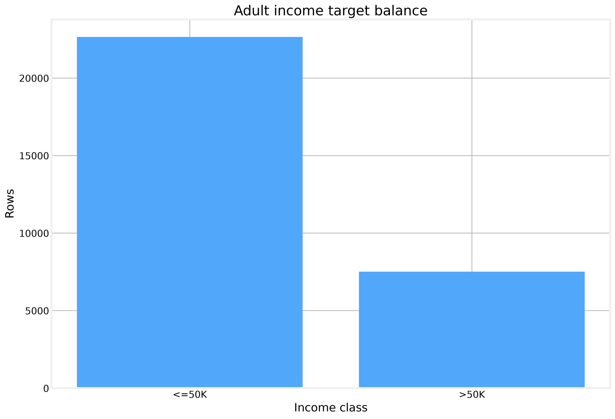
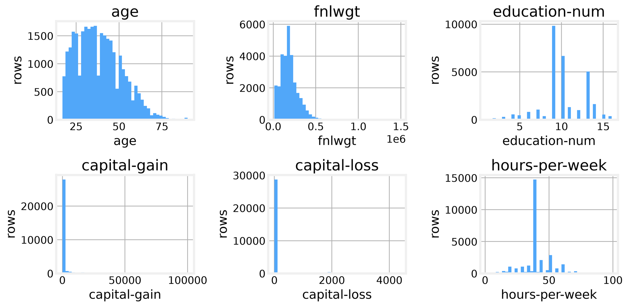
The target balance is the first thing that matters. Only 24.9 percent of rows earn over 50K, which means any model that predicts the majority class every time would look accurate while missing most of the interesting cases. The numeric fields show heavy right skew in capital-gain and capital-loss, with thousands of zeros and a long tail of large values. Tree models will handle this fine, but it tells us not to expect linear relationships to carry the day.

The correlation heatmap confirms no numeric feature is a near-duplicate of another, and the categorical distributions show the usual long tails: workclass has a dominant Private category, education spans sixteen levels, and native-country is mostly United-States with a thin spread of others. These observations drive everything that follows, from stratified validation to the choice of tree-based models.

Regression metrics

Before we classify income, we grade a tiny regression task on the same table: predict age from four numeric census features. This makes the five core regression metrics concrete without adding a second dataset.

All five metrics compare predicted ages with true ages. Mean Squared Error (2) punishes large errors disproportionately, Root Mean Squared Error (2) brings the number back into years, Mean Absolute Error (2) tolerates outliers, Mean Absolute Percentage Error (2) reports a percentage, and R-squared (2) compares our model with the mean baseline.

The mean baseline predicts the average age for everyone and lands at an RMSE of 12.98 years. A linear regression on education-num, hours-per-week, capital-gain, and capital-loss improves that to 12.85 years. The gap is 0.13 years, which tells us these four features barely move the needle on age prediction. R-squared confirms the story at 0.020, meaning the features explain about two percent of age variance. The lesson is not that regression metrics are weak, but that they give us a precise language for saying how weak a model is.

Ranking metrics

Those regression metrics need a continuous target; our income target is binary, so we turn to ranking metrics. Ranking metrics matter whenever a model outputs scores rather than labels, and we use a small synthetic search example to see NDCG (3), Mean Reciprocal Rank (3), and Mean Average Precision (3) in action.

The idea behind all three is simple: when a model ranks documents or products, we care where the relevant items land. Mean Reciprocal Rank (3) rewards the first relevant hit, giving 1.0 if the top result is relevant, 0.5 if the second is, and so on. Mean Average Precision (3) averages precision at each relevant hit, which rewards getting many relevant items high in the list. NDCG (3) generalizes this to graded relevance, where some items are more relevant than others, and normalizes by the best possible ordering.

Our synthetic example has two queries with known relevant documents. The rankings place the relevant items first in both cases, so MRR and MAP both score 1.000. The NDCG example uses graded relevance from 3 down to 0, and a perfect ordering scores 1.000 as well. These metrics matter for search and recommendation, and they will matter again when we evaluate probability scores rather than hard predictions.

Validation habits

Now we build the income classifier on a random 20,000-row subsample of the cleaned table. The full 30,139 rows would make six search experiments slow on a CPU, so we draw the subsample once with seed 42 and split it into 15,000 training rows and 5,000 test rows. The test set stays untouched until the final headline cell.